Inference with Mathematical Models

IMS1 Ch. 13
Math 215

Yurk

Opportunity Costs

Research question: Does reminding someone of opportunity cost impact purchase decision?
opportunity_cost ¹ dataset
2 variables
- group: treatment or control
- decision: buy or not buy
150 students (75 assigned to treatment, 75 control)

All students given the following statement:

“Imagine that you have been saving some extra money on the side to make some purchases, and on your most recent visit to the video store you come across a special sale on a new video. This video is one with your favorite actor or actress, and your favorite type of movie (such as a comedy, drama, thriller, etc.). This particular video that you are considering is one you have been thinking about buying for a long time. It is available for a special sale price of $14.99. What would you do in this situation? Please circle one of the options below.”

Control and treatment group given different options.

Control

“(A) Buy this entertaining video. (B) Not buy this entertaining video.”

Treatment

“(A) Buy this entertaining video. (B) Not buy this entertaining video. Keep the $14.99 for other purchases.”

group	buy video	not buy video	total
treatment	41	34	75
control	56	19	75
total	97	53	150

Standardized barplot showing proportions of students that buy or do not buy

Difference in proportions

Success: decision = “not buy video”
Statistic of interest: difference in proportions \[\hat{p}_T-\hat{p}_C\]
Observed difference: \[\frac{34}{75}-\frac{19}{75}=0.2\]

Hypotheses

In words:

    $H_0:$ How the options are
    presented has no impact
    on decision.

    $H_A:$ Higher proportion
    will choose not to buy if
    opportunity cost
    highlighted.

In symbols:

$H_0: p_T -p_C = 0$
$H_A: p_T -p_C > 0$

Null Distribution - Simulation

Simulate 1,000 samples assuming true null hypothesis
Random permutation of response (decision)
Calculate statistic for each permutation
Use infer package

library(infer)
opportunity_perm <- opportunity_cost |>
  specify(decision ~ group, success = "not buy video") |>
  hypothesize("independence") |>
  generate(reps = 1000, type = "permute") |>
  calculate(stat = "diff in props", order = c("treatment", "control"))

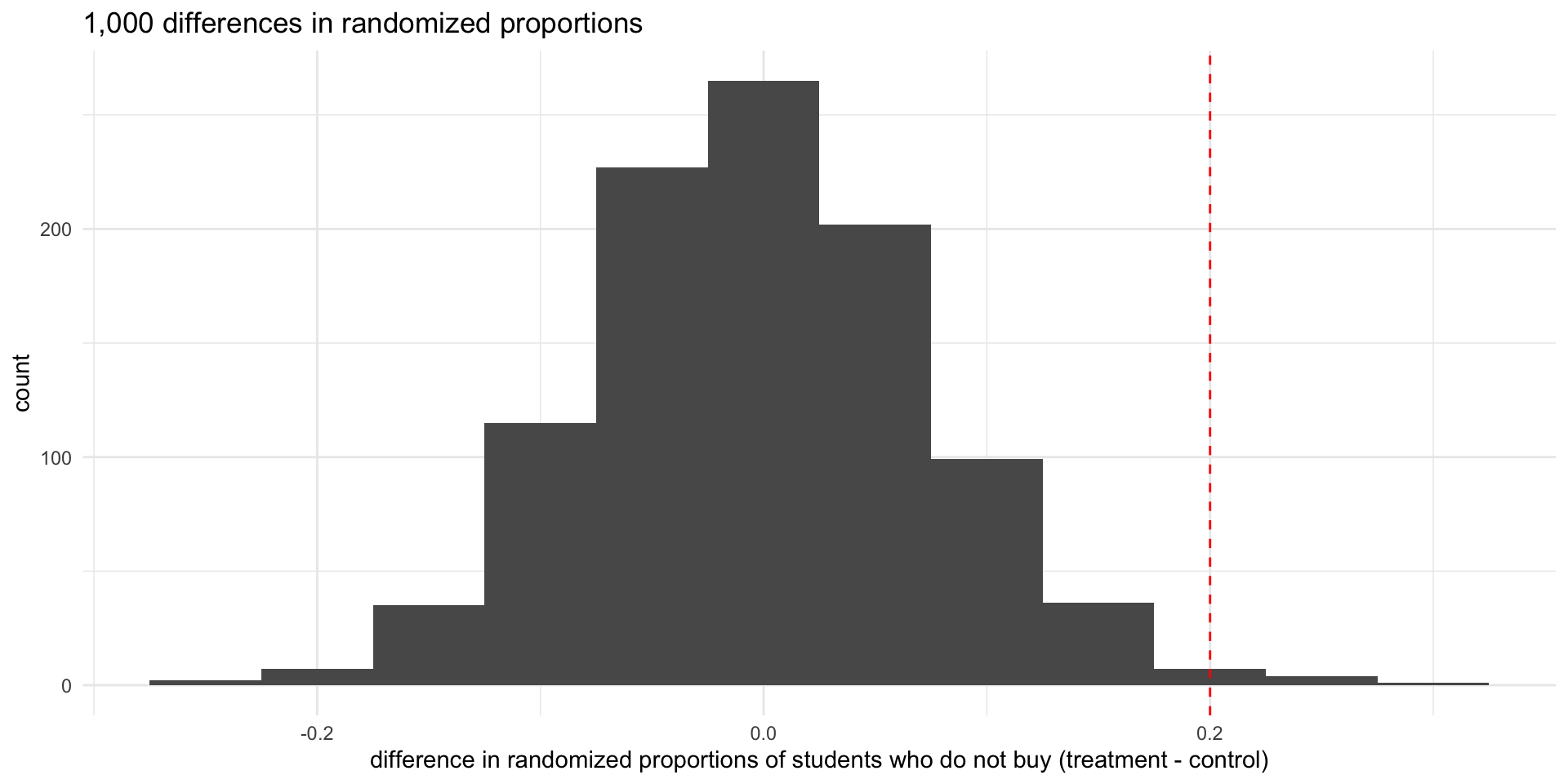
Histogram of 1,000 differences in randomized proportions (null distribution), showing observed difference as dashed vertical line.

p-value - Simulation

The p-value is the probability that the value of the statistic would be at least as extreme as the observed value if the null hypothesis is true
Out of 1,000 simulations of a true null hypotheses, 5 had differences $\hat{p}_T-\hat{p}_C \geq 0.2.$
Thus, the p-value is $\frac{5}{1000} = 0.005$

opportunity_perm |>
  summarize(ext_count = sum(stat >= 0.2),
            pval = mean(stat >= 0.2))

# A tibble: 1 × 2
  ext_count  pval
      <int> <dbl>
1         5 0.005

Standard error - Simulation

We can also use the null distribution to compute a standard error (standard deviation of a sampling distribution)
$SE = 0.0797$

opportunity_perm |>
  summarize(SE = sd(stat))

# A tibble: 1 × 1
      SE
   <dbl>
1 0.0797

Null Distribution – Mathematical Model

It may be possible to use a mathematical model of the null distribution instead of simulation
For a single proportion or difference in proportions, we may be able to use a normal distribution

Central Limit Theorem for proportions

The sample proportion (or difference in proportions) will follow a bell-shaped curve called the normal distribution if the following technical conditions are met:

independent observations
large enough sample: for proportions, at least 10 successes and 10 failures in each group

Normal Distributions

$N(\mu, \sigma)$ denotes a normal distribution with mean $\mu$ and standard deviation $\sigma$

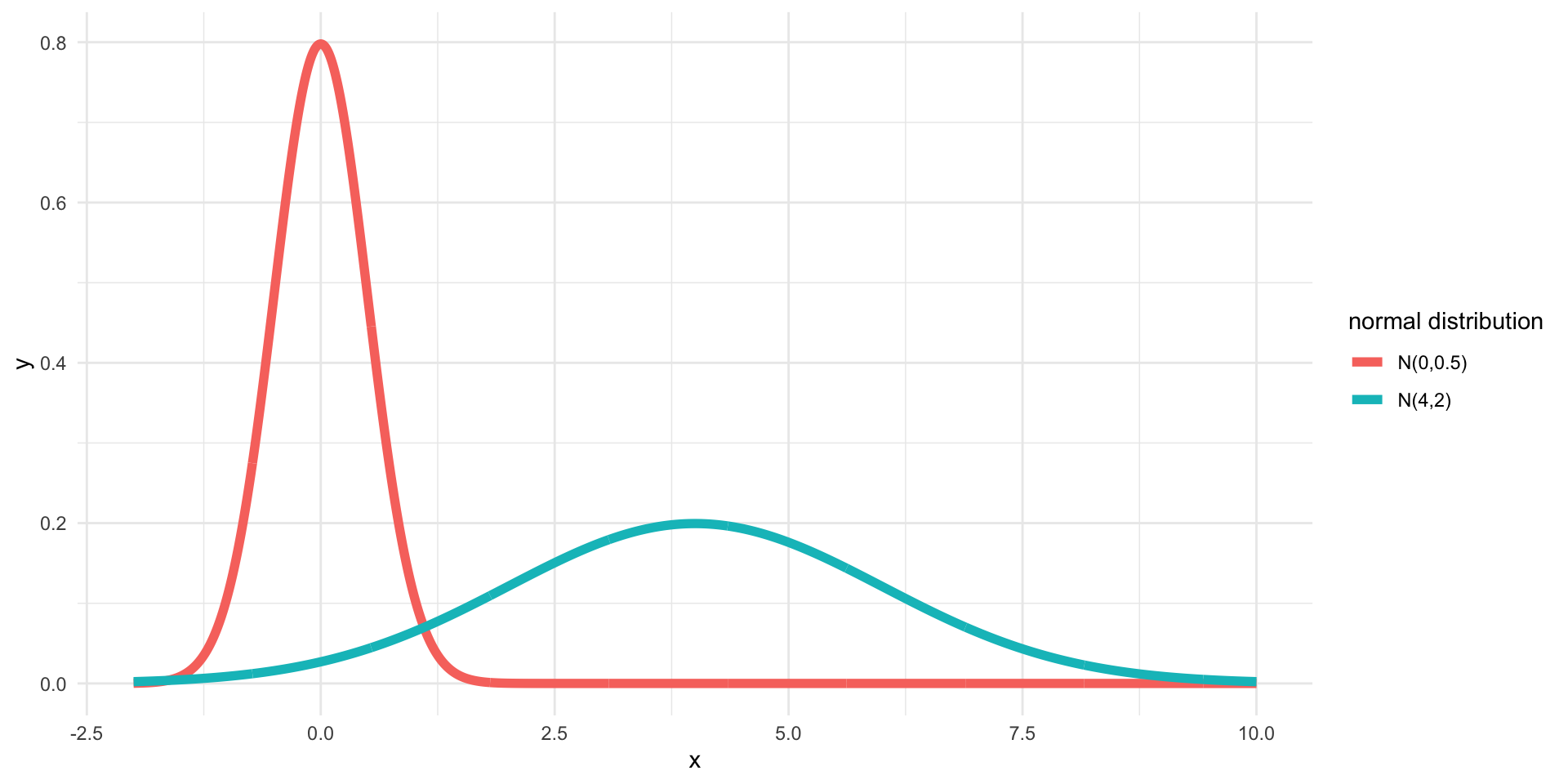
Two examples of normal distributions with different means and standard deviations

Normal Approximation of Null Distribution

The data in the opportunity cost example satisfy the techincal conditions
We can approximate the null distribution using $N(\mu = 0, \sigma = 0.0797)$
Why would we use these values?

How good is the approximation?

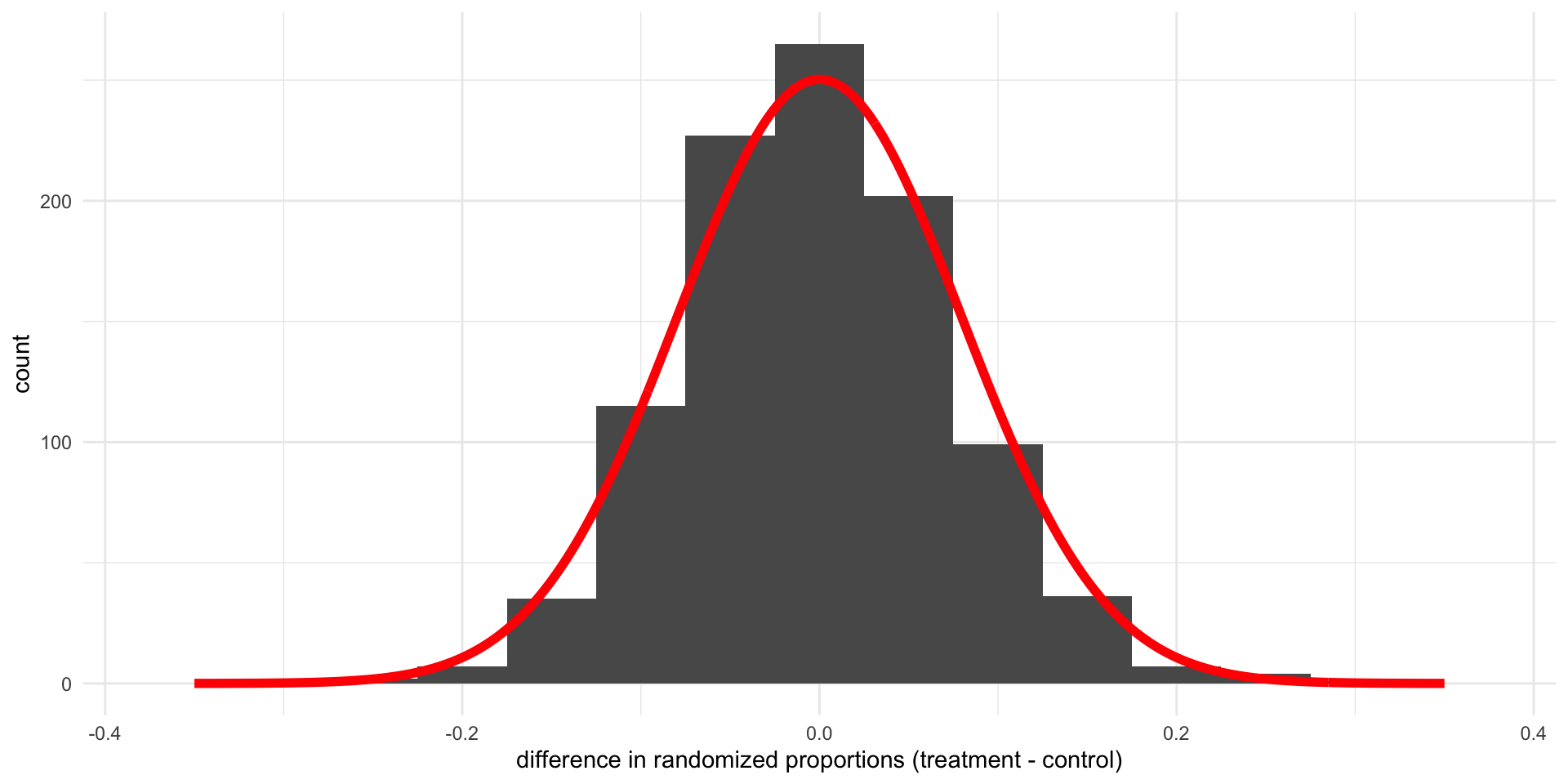
Null distribution from rondomly permuted data and normal approximation

Computing Probabilities Using a Normal Distribution

For a probability density function, the area under the curve (integral) is a probability

Shaded area is probability that value is less than 0.1

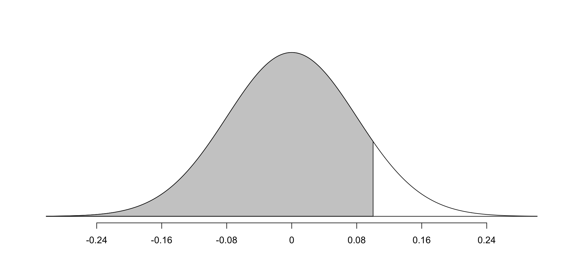
The probability that the value is less than 0.1 is

pnorm(0.1, mean = 0, sd = 0.0797)

[1] 0.8952071

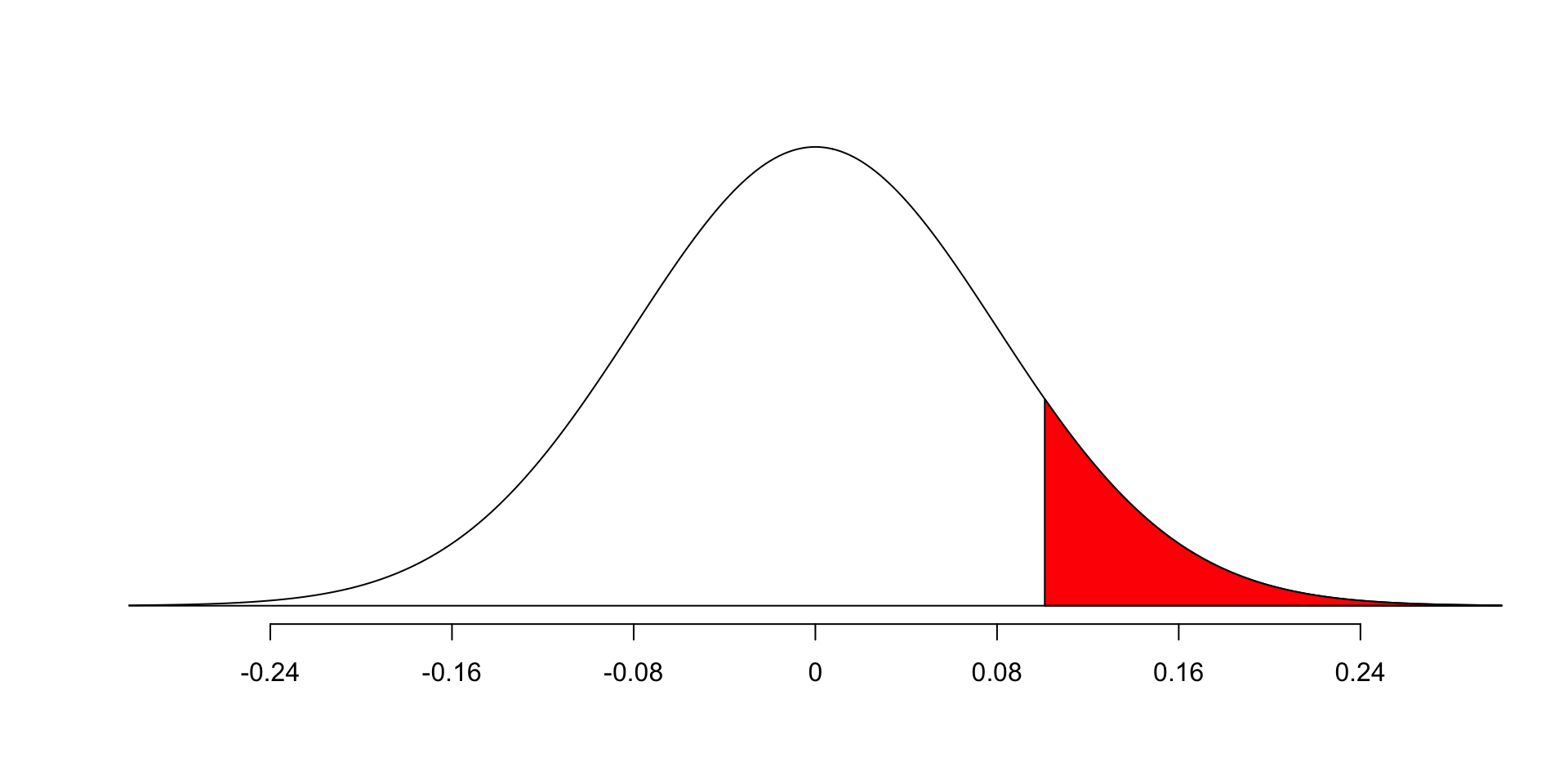
The probability that the value is at least 0.1 is

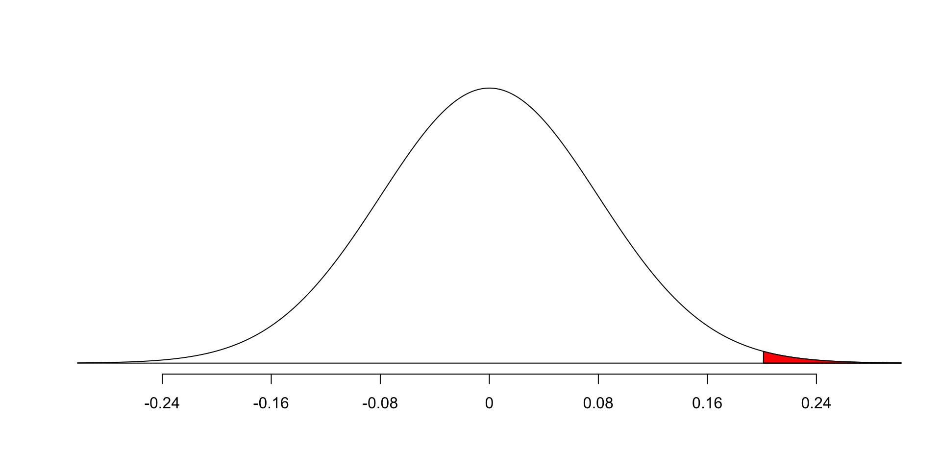
1 - pnorm(0.1, mean = 0, sd = 0.0797)

[1] 0.1047929

Computing a p-value from a Normal Distribution

We can compute a p-value using the normal approximation of the null distribution
Find the area in the tail is beyond the observed value of the statistic

The p-value is

1 - pnorm(0.2, mean = 0, sd = 0.0797)

[1] 0.006046646

Z score

The Z score of an observation is the number of standard deviations that the observation falls above or below the mean. \[Z = \frac{x-\mu}{\sigma}\]

We can standardize the observed difference in proportions in the opportunity costs problem \[Z = \frac{0.2 - 0}{0.0797} = 2.509\]

If the $X$ is distributed according to $N(\mu,\sigma)$, then $Z$ will be distributed according to $N(0,1)$
$N(0,1)$ is called the standard normal distribution

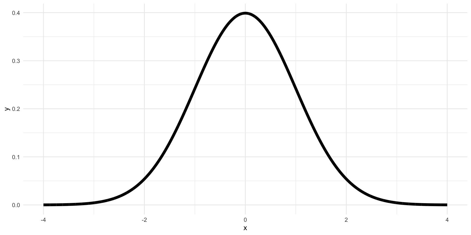
Standard normal distribution

We can use the Z score to calculate the p-value using the standard normal distribution

z = (0.2 - 0)/0.0797
1 - pnorm(z, mean = 0, sd = 1)

[1] 0.006046646

68-95-99.7 rule

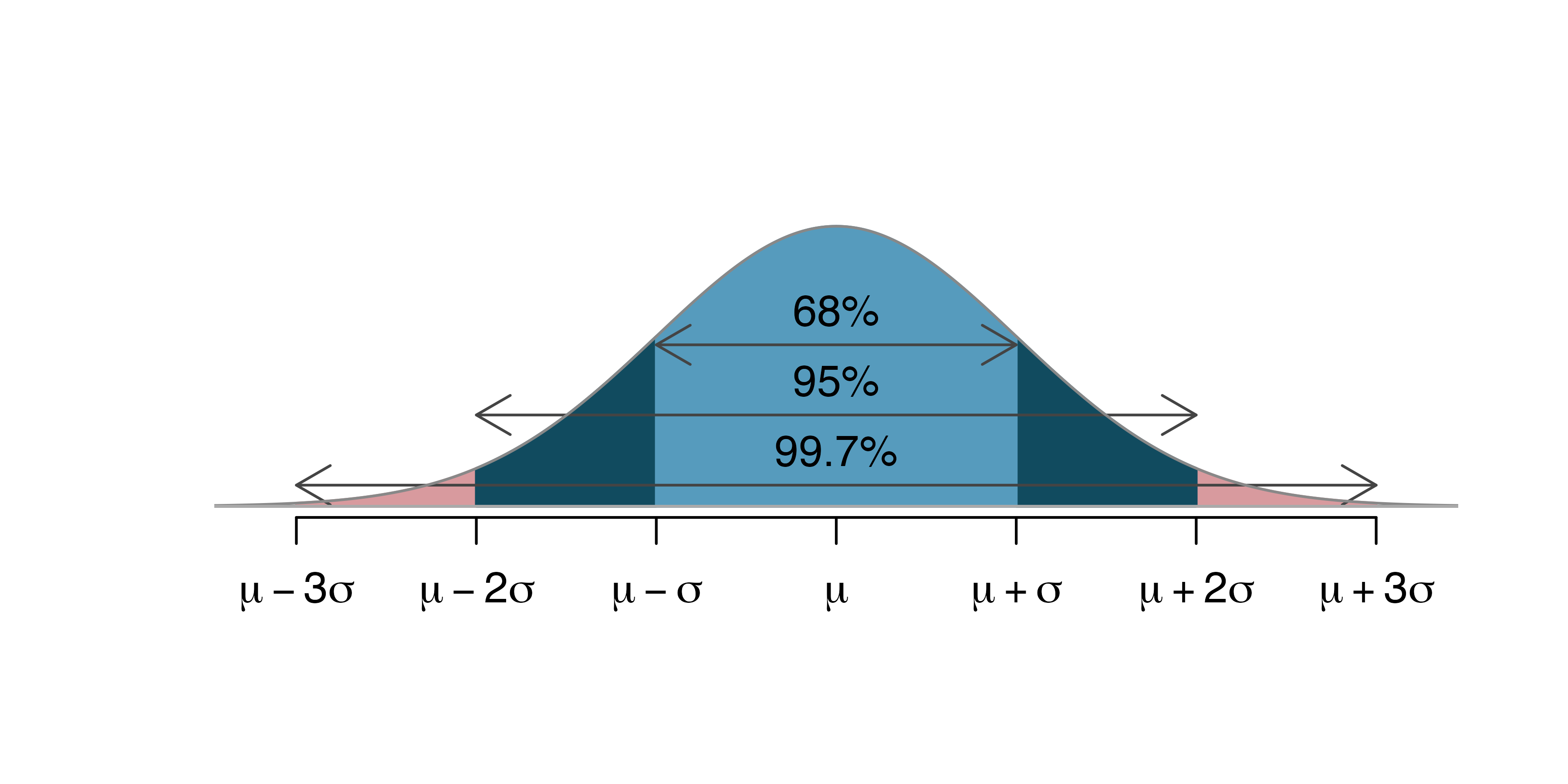
From IMS1 Figure 13.8.

About 68% of normally distributed data fall within 1 SD of the mean
About 95% fall within 2 SD (1.96 to be more precise)
About 99.7% fall within 3 SD

This rule can be used to bound p-values
If Z = 2.509, we know the value is outside of the middle 95% of the distribution
Thus it is some where in the right tail that includes 2.5% of the data
This means we know the p-value is less than 0.025, just based on the Z score

Using a Normal Distribution to Construct a 95% Confidence Interval

If sampling distribution is reasonably normal then we can construct a 95% confidence interval from a point estimate using the 68-95-99.7 rule
95% of the values will fall within 1.96 SD of the true value
95% confidence interval: \[\textrm{point estimate}\pm1.96\times SE\]

0.2 is a point estimate of the difference in proportions of students who would not buy a video ($p_T-p_C$)
SE = 0.0797
A 95% confidence interval for the difference in proportions is \[0.2 \pm 1.96\times0.0797 = 0.2 \pm 0.156\]
The quantity 0.156 is called the margin of error
We can also write the 95% confidence interval as $(0.0438, 0.356)$

Other Confidence Levels

For other confidence levels, the confidence interval can be computed as \[\textrm{point estimate}\pm z^{\ast}\times SE\]
To determine $z^{\ast}$, need to know how many standard deviations needed to contain X% of the data, where X% corresponds to the confidence level

qnorm give us the cutoff value where the area under the curve up to the cuttoff is equal to the desired value
For a 99% CI, we want to find the cuttoff that includes 99.5% of the values, leaving 0.5% in the right tail

qnorm(0.995, mean = 0, sd = 1)

[1] 2.575829

Thus, a 99% CI for the difference in proportions is \[0.2\pm 2.58 \times 0.0797=0.2 \pm 0.205\]
Note that the margin of error is larger with a higher confidence level

What is the value of $z^{\ast}$ for a 95% CI?

qnorm(0.975, mean = 0, sd = 1)

[1] 1.959964

90%?

qnorm(0.95, mean = 0, sd = 1)

[1] 1.644854