Confidence Intervals:One proportion
Topic 4
Math 115
Math 115
Two Types of Questions
Hypothesis Testing: Is a specific value plausible?
- Medical consultant: “Is her complication rate different from 10%?”
- We tested \(H_0: p = 0.10\)
- Answer: Reject or fail to reject \(H_0\)
- When we failed to reject the null hypothesis, we imply that in a long run it is plausible that the true complication rate of this physician could be 0.1
Today (Confidence Intervals): Are there other values that are plausible?
- “What IS the complication rate?” (not just testing one value)
- Answer: An interval estimate
Point Estimates and Their Limitations
From hypothesis testing, we know:
- \(\hat{p}\) is our best single guess for \(p\)
- But different samples give different values of \(\hat{p}\) (sampling variability)
- A single number doesn’t express our uncertainty
Solution: Use an interval estimate instead of just a point estimate
- Expresses a range of plausible values for \(p\)
- This is called a confidence interval
Sampling Distribution
- We can estimate the variabilty in the population by constructing sampling distribution
- A sampling distribution is the distribution we would obtain if we could select samples of the same sample size again and again from the same population, calculating the value of the statistic of interest each time
- Much of inferential statistics is based on being able to approximate sampling distributions
- We rarely have the ability to select many samples from the same population (if we did we would usually just select a larger sample!)
- However, we can make up a population and repeatedly sample from it to test different statistical ideas
Candidate X
Context: Candidate X is running for mayor. Her campaign wants to estimate the proportion of all voters who support her.
Data: Campaign polls a random sample of 30 voters
- 21 people support Candidate X
- \(\hat{p} = \frac{21}{30} = 0.7\) (70%)
Point estimate: About 70% of all voters support her
Question: How confident should we be in this estimate?
The Challenge
We want to know how much \(\hat{p}\) varies from sample to sample.
In hypothesis testing:
- We simulated from a spinner assuming \(p = 0.10\) (the null hypothesis)
- This gave us the null distribution
- Showed what we’d see if \(H_0\) were true
Now we have a problem:
- We don’t know \(p\) (that’s what we’re trying to estimate!)
- Can’t build a spinner without knowing \(p\)
- Need a different approach…
Our Best Information
Key insight: Our sample is the best approximation we have of the population
- If 70% of our sample supports Candidate X, that’s our best guess about the population
- The sample reflects the population (at least approximately)
The bootstrap idea: Use our sample as a stand-in for the population
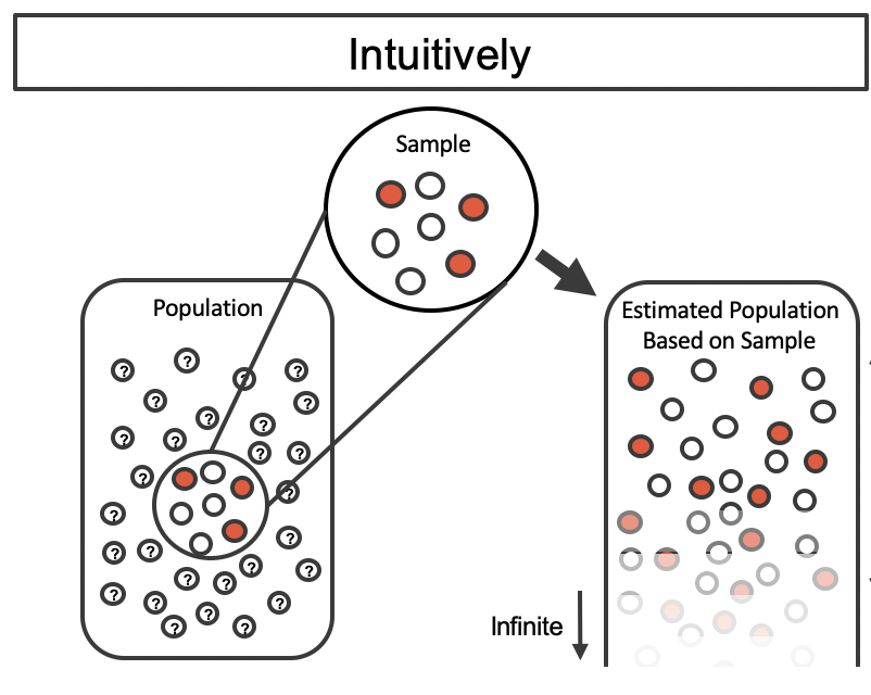
A single sample
A comparison of the process of sampling from the estimate infinite population and resampling with replacement from the original sample.(Fugure 12.1 from IMS2)
Bootstrap Sampling
Realistically, we don’t have the entire population to take samples from. We only have one sample and want to use it to construct the sampling distribution
Bootstrap sample: Sample WITH replacement from the original sample
- Same size as original (n = 30)
- “With replacement” = same observation can appear multiple times
- Each bootstrap sample is slightly different from original
Example bootstrap sample:
- Might select ID #5 three times, ID #12 twice, ID #18 zero times
- Creates natural variation
Resampling with Replacement
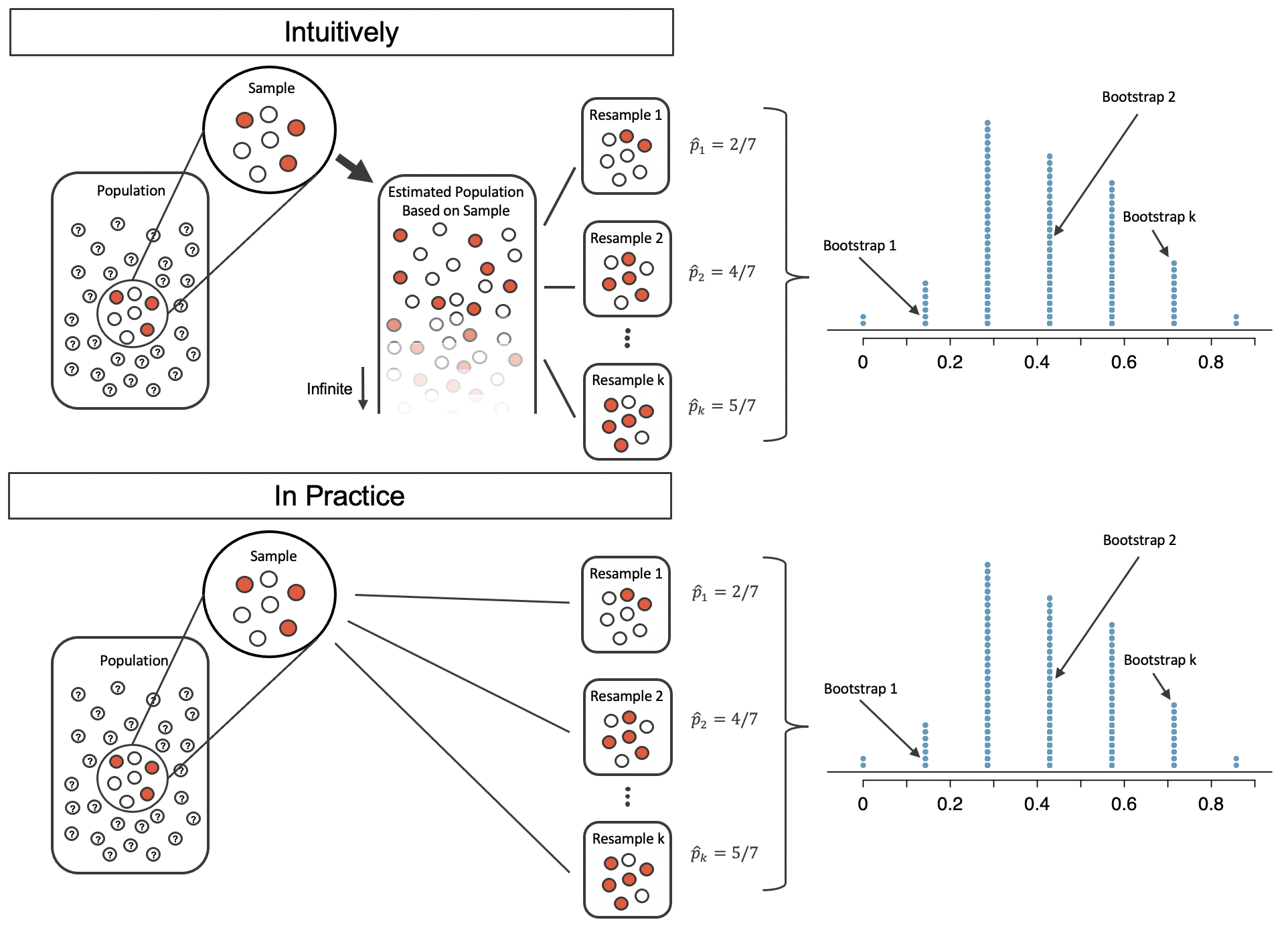
Five bootstrapped samples
Building the distribution
The logic:
- Our sample reflects the population structure
- Resampling with replacement recreates the “luck of the draw”
- This variation approximates how \(\hat{p}\) varies across samples
- Key: We’re NOT assuming any particular value of \(p\)
Compare to hypothesis testing:
- Hypothesis testing: assumed \(p = 0.10\), simulated what that would look like
- Confidence intervals: use actual data, no assumption about \(p\)
Bootstrap vs Randomization
Hypothesis Testing
- Simulated from spinner at \(p_0 = 0.10\)
- Assumed \(H_0\) is TRUE
- Distribution centered at 0.10
- Answers: “Is 0.10 plausible?”
Confidence Intervals
- Resample from actual data
- No assumption about \(p\)
- Distribution centered at \(\hat{p} = 0.7\)
- Answers: “What values are plausible?”
Same concept (simulation for variability), different purpose
Interactive Bootstrap Demo
Try the interactive simulation:
- Run 1 sample at a time and watch the resampling animation
- Run 100 samples to quickly build the bootstrap distribution
- See how bootstrap proportions stack up in the dotplot
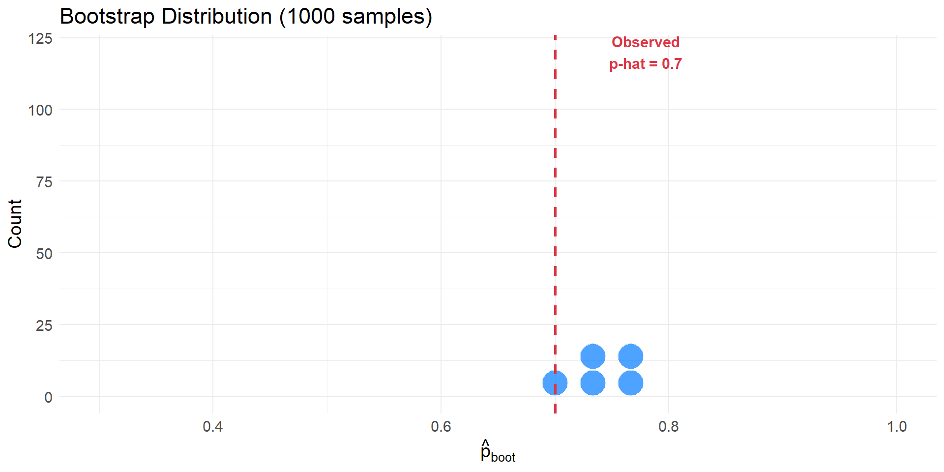
1000 Bootstrapped Proportions
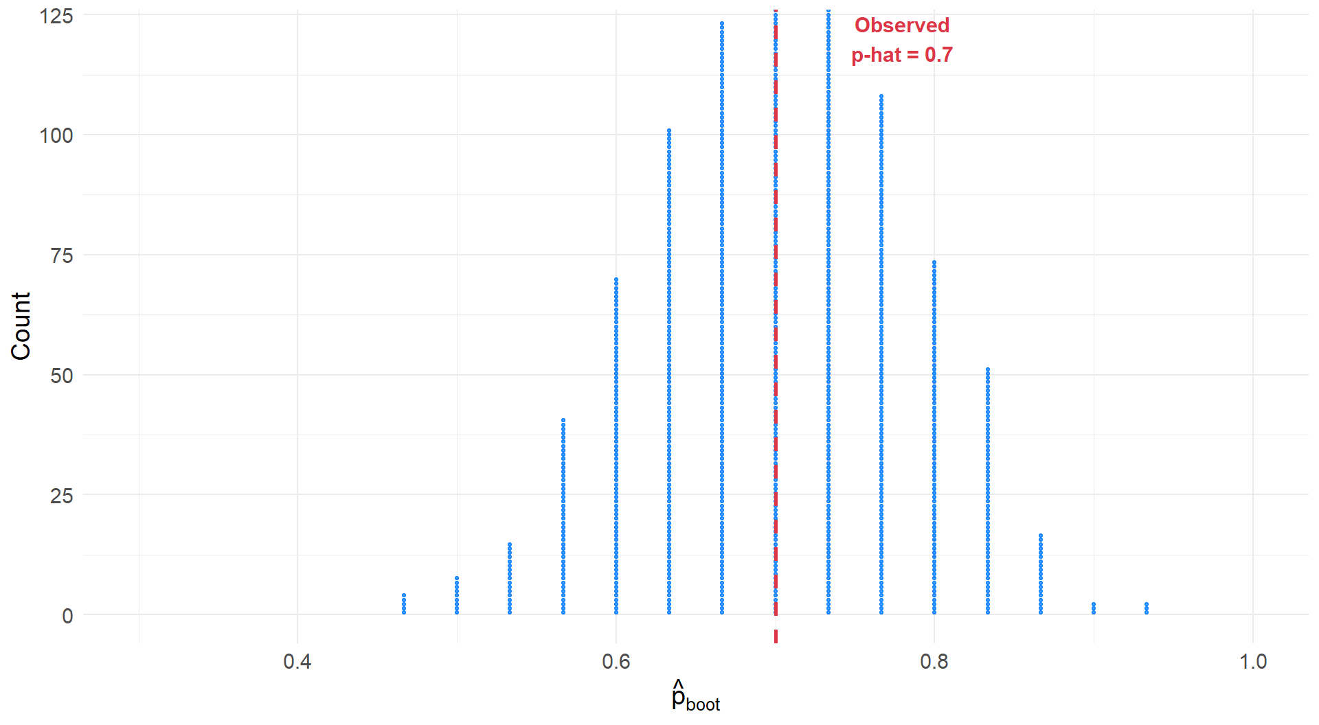
Building the Bootstrap Distribution
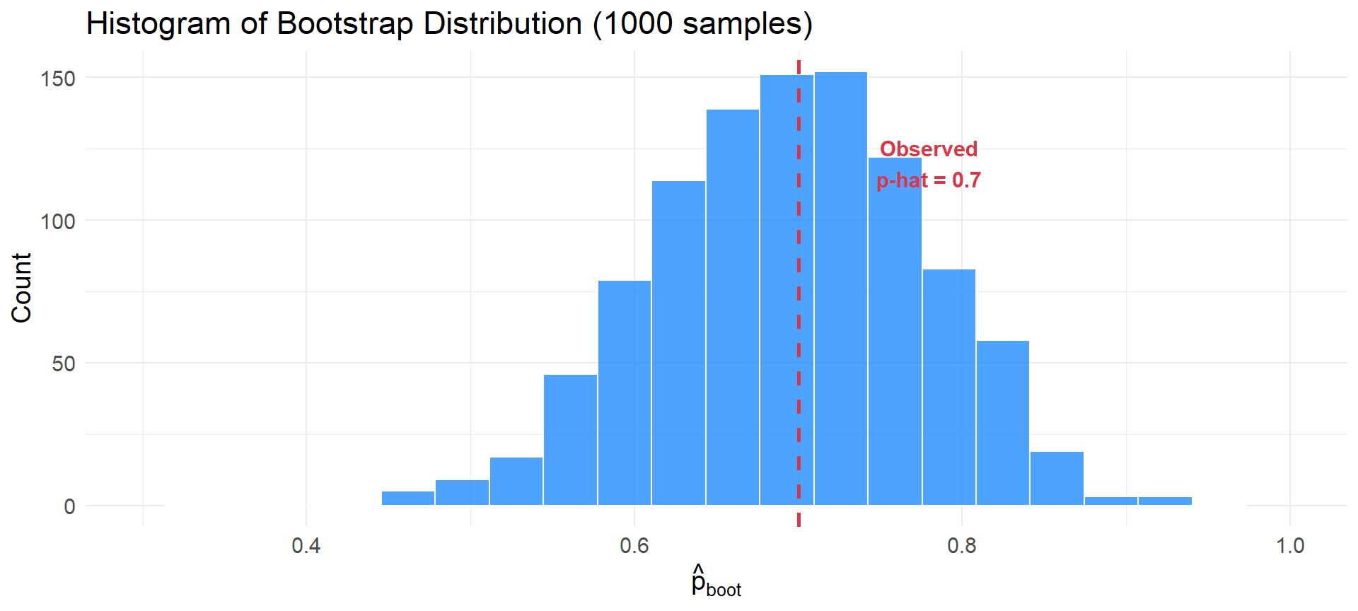
Histogram of 1000 bootstrap proportions. Distribution centered near 0.7 (our observed \(\hat{p}\)).
Bootstrap Standard Error
Standard Error (SE): Standard deviation of a statistic (in this case \(\hat{p}\))
- Measures uncertainty in our estimate
- For Candidate X: \(SE_{boot} = 0.082\)
Interpretation: The measure of the spread of \(\hat{p}\) is about 0.082
The Percentile Method
To create a 95% confidence interval:
- Take the bootstrap distribution
- Find the middle 95% of values
- Cutoffs: 2.5th percentile and 97.5th percentile
Why these percentiles?
- 2.5% below, 95% in the middle, 2.5% above
- These values “fence in” the middle 95%
Computing the 95% CI
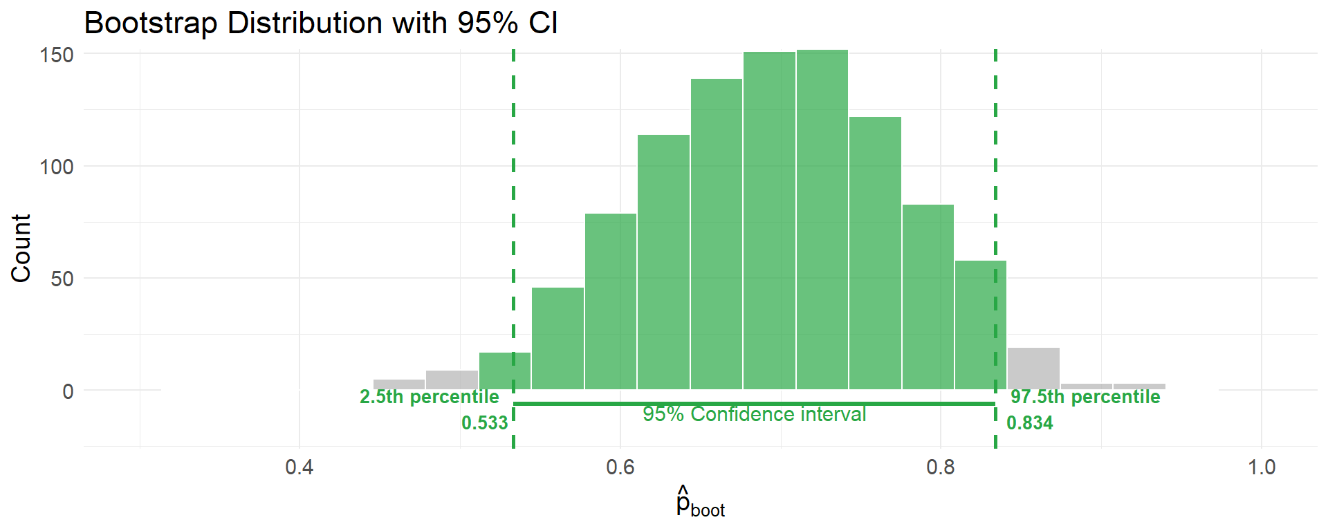
95% Confidence Interval: (0.533, 0.834)
Interpreting Confidence Intervals
Our 95% CI for Candidate X: (0.533, 0.834)
Correct interpretation:
“We are 95% confident that the true proportion of voters who support Candidate X is between 0.533 and 0.834.”
What this means:
- Values inside the interval are plausible for \(p\)
- Values outside the interval are implausible for \(p\)
- For example, it is plausible that 80% of people plan to vote for Candidate X.
- It is not plausible that 50% (or less) of people plan to vote for Candidate X.
- This would be good news for Candidate X.
What Does “95% Confident” Mean?
Common Misinterpretation
❌ WRONG: “There is a 95% probability that \(p\) is in this interval”
✅ CORRECT: “We are 95% confident that this interval contains \(p\)”
Why the distinction?
- The parameter \(p\) is fixed (but unknown)
- It either is or isn’t in our interval
- The 95% refers to our confidence in the method, not probability about this specific interval
If we repeated this process many times using new samples of 30, about 95% of intervals would contain \(p\)
95% vs 99% Confidence intervals
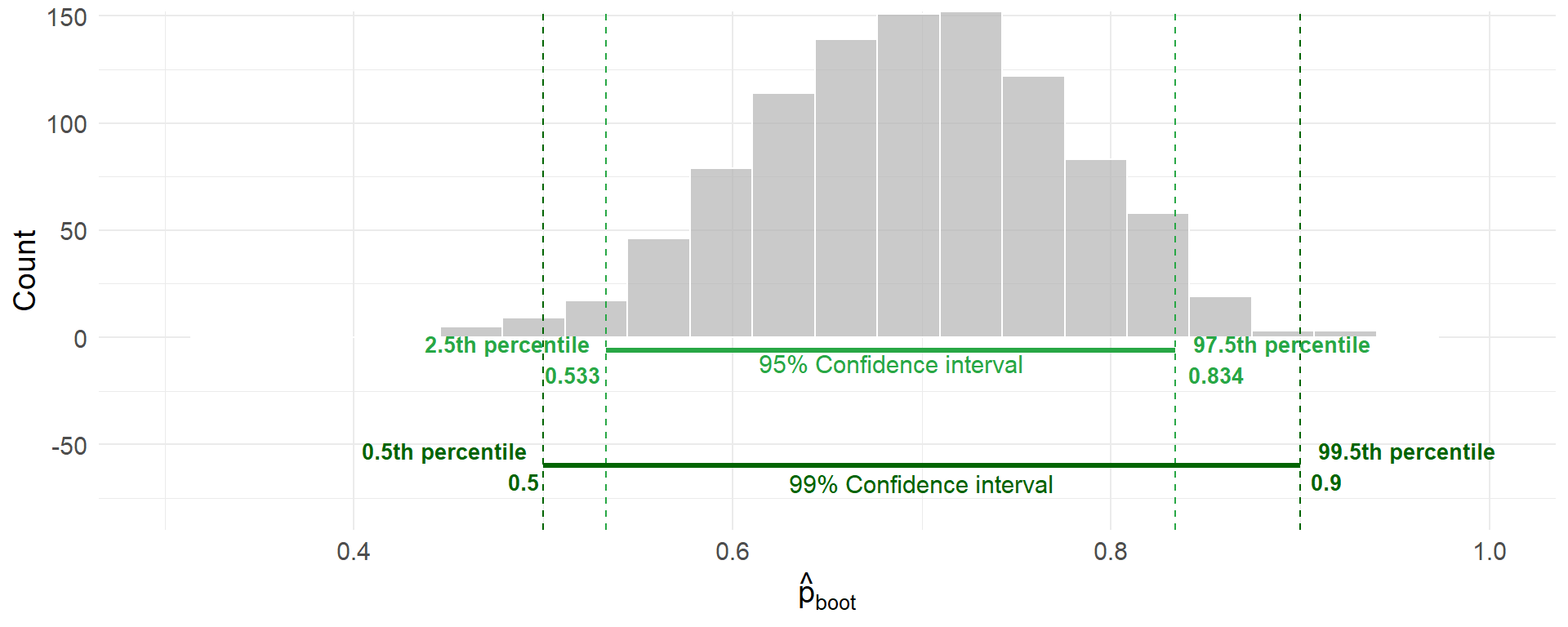
95% Confidence Interval: (0.533, 0.834)
99% Confidence Interval: (0.5, 0.9)
Properties of Confidence Intervals
Three key properties:
- CI contains the observed statistic (usually near the center)
- Our CI for Candidate X is centered near \(\hat{p} = 0.7\)
- Larger sample → narrower CI (more precision)
- n = 30 gives wider interval than n = 300 would
- Higher confidence level → wider CI (more conservative)
- 99% CI is wider than 95% CI
Other Confidence Levels
For Candidate X bootstrap distribution:
| Confidence Level | Percentiles | Interval |
|---|---|---|
| 90% | 5th to 95th | (0.567, 0.833) |
| 95% | 2.5th to 97.5th | (0.533, 0.834) |
| 99% | 0.5th to 99.5th | (0.5, 0.9) |
Notice: Higher confidence → wider interval
Trade-off: Confidence vs. Precision
Connecting to Hypothesis Testing
Let’s revisit the medical consultant from hypothesis testing:
Data: 3 complications in 62 surgeries, \(\hat{p} = 0.048\)
Bootstrap 95% CI: (0, 0.113)
Key observation: The national rate of 0.10 IS in this interval
Connection to hypothesis testing: We failed to reject \(H_0: p = 0.10\) (p-value = 0.11)
Insight: Values in the CI are exactly those we would NOT reject in a (two-sided) hypothesis test!
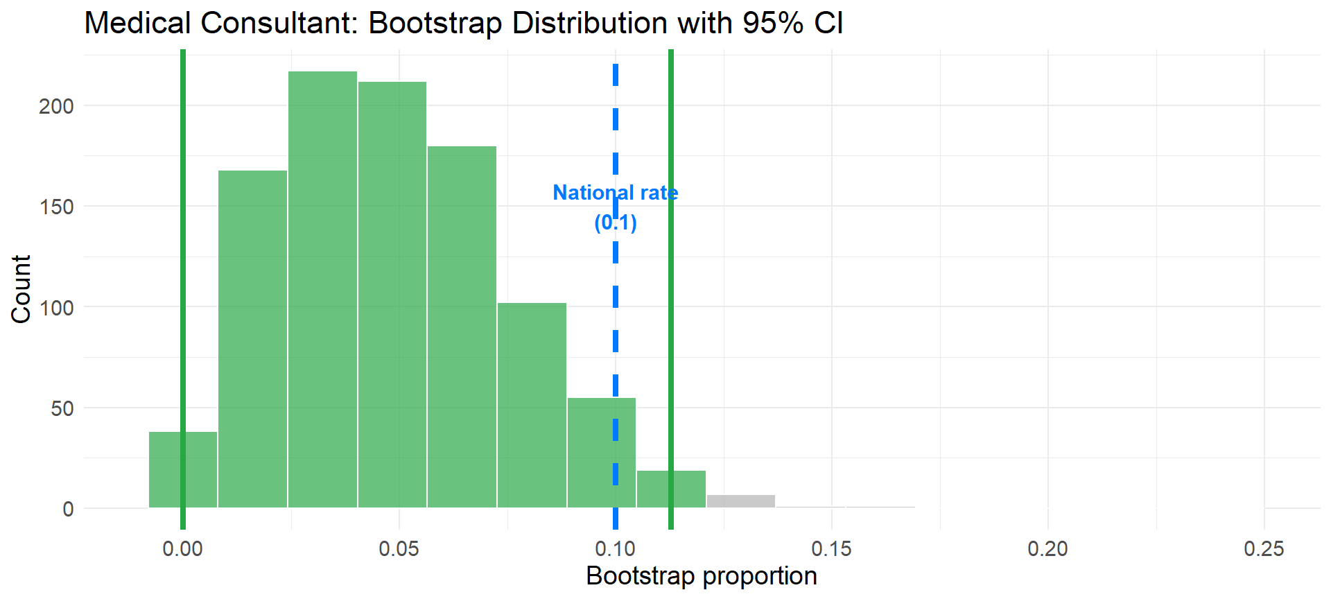
The national rate (0.10) falls within the 95% CI—consistent with our hypothesis test result.
The Confidence Interval Process
Summary of steps:
Collect sample and calculate \(\hat{p}\)
Generate bootstrap samples: Resample with replacement (at least 1000 times)
Calculate \(\hat{p}_{boot}\) for each bootstrap sample
Build bootstrap distribution from all bootstrap proportions
Find percentiles: 2.5th and 97.5th for 95% CI
Interpret in context: “We are 95% confident that \(p\) is between…”
Bootstrap vs H-Test Randomization Summary
| Feature | Hypothesis Testing | Confidence Intervals |
|---|---|---|
| Question | Is \(p_0\) plausible? | What values of \(p\) are plausible? |
| Method | Simulate \(H_0\) | Bootstrap resampling from original data with replacement |
| Assumes | \(H_0\) is true (\(p = p_0\)) | Nothing about \(p\) |
| Distribution centered at | \(p_0\) (null value) | \(\hat{p}\) (observed value) |
| Output | P-value | Confidence interval |
| Decision | Reject / Fail to reject \(H_0\) | Values in / out of CI |
Both methods: Use simulation to understand sampling variability, but for different purposes
References
- Introduction to Modern Statistics (2e) textbook by Mine Cetinkaya-Rundel and Johanna Hardin
- Chapter 12: Confidence Intervals with Bootstrapping