Inference: Regression Single Predictor

Chapter 24
Math 115

Body Measurements

bdims body measurement dataset is available here.
507 physically active individuals (247 men, 260 women)
age, weight (wgt), height (hgt), sex, 21 body girth variables (e.g., hip girth)

Regression Line

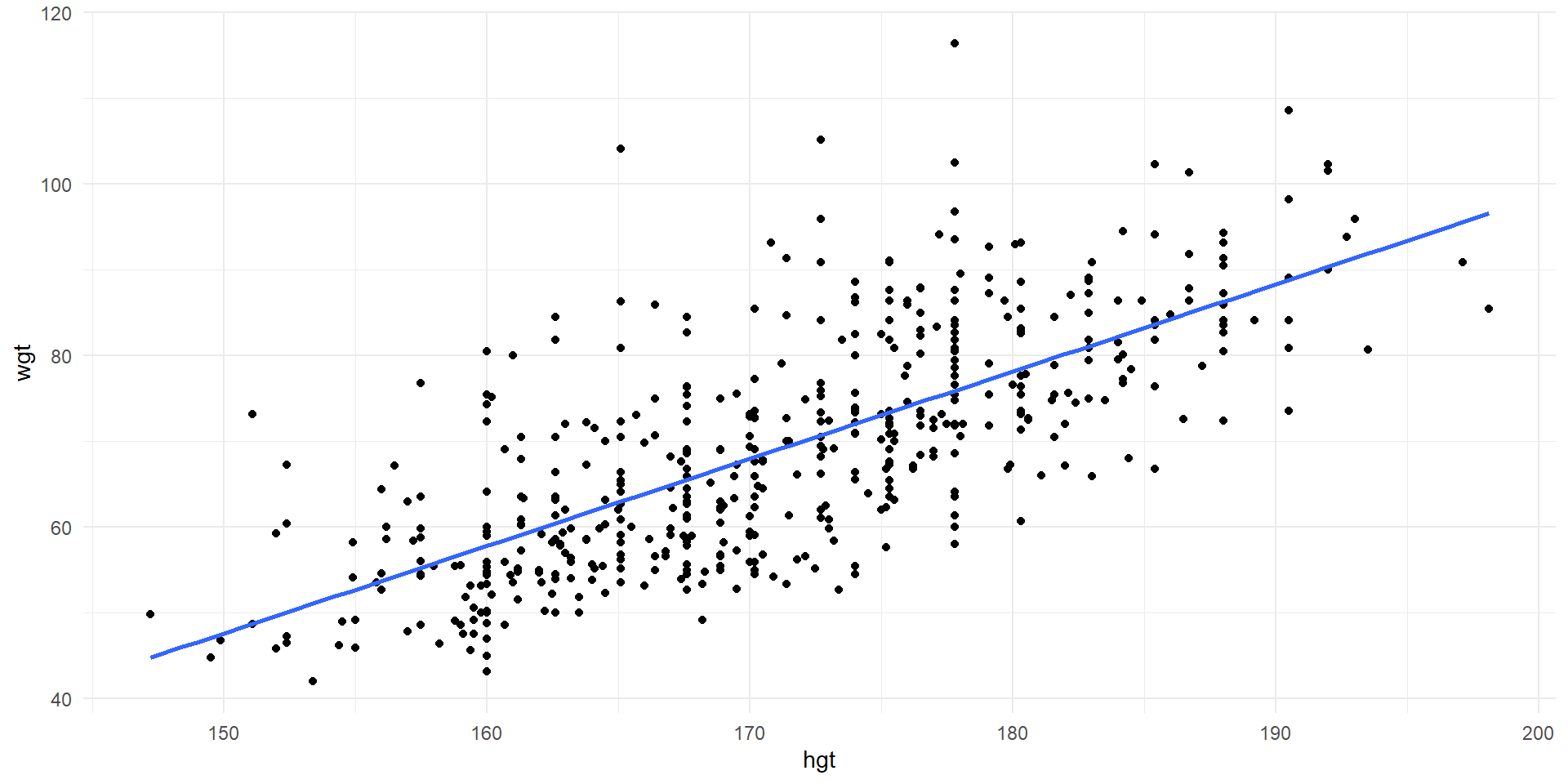
Observations of wgt vs. hgt and least squares line for the entire population.

Least squares regression line (Recall from Chapter 7) \[\widehat{Weight}=-105.01+1.02\times Height\]

Variability in Slopes

Slope can vary from sample to sample from the same population
We will explore this variability with random samples of 20 individuals from the bdims data

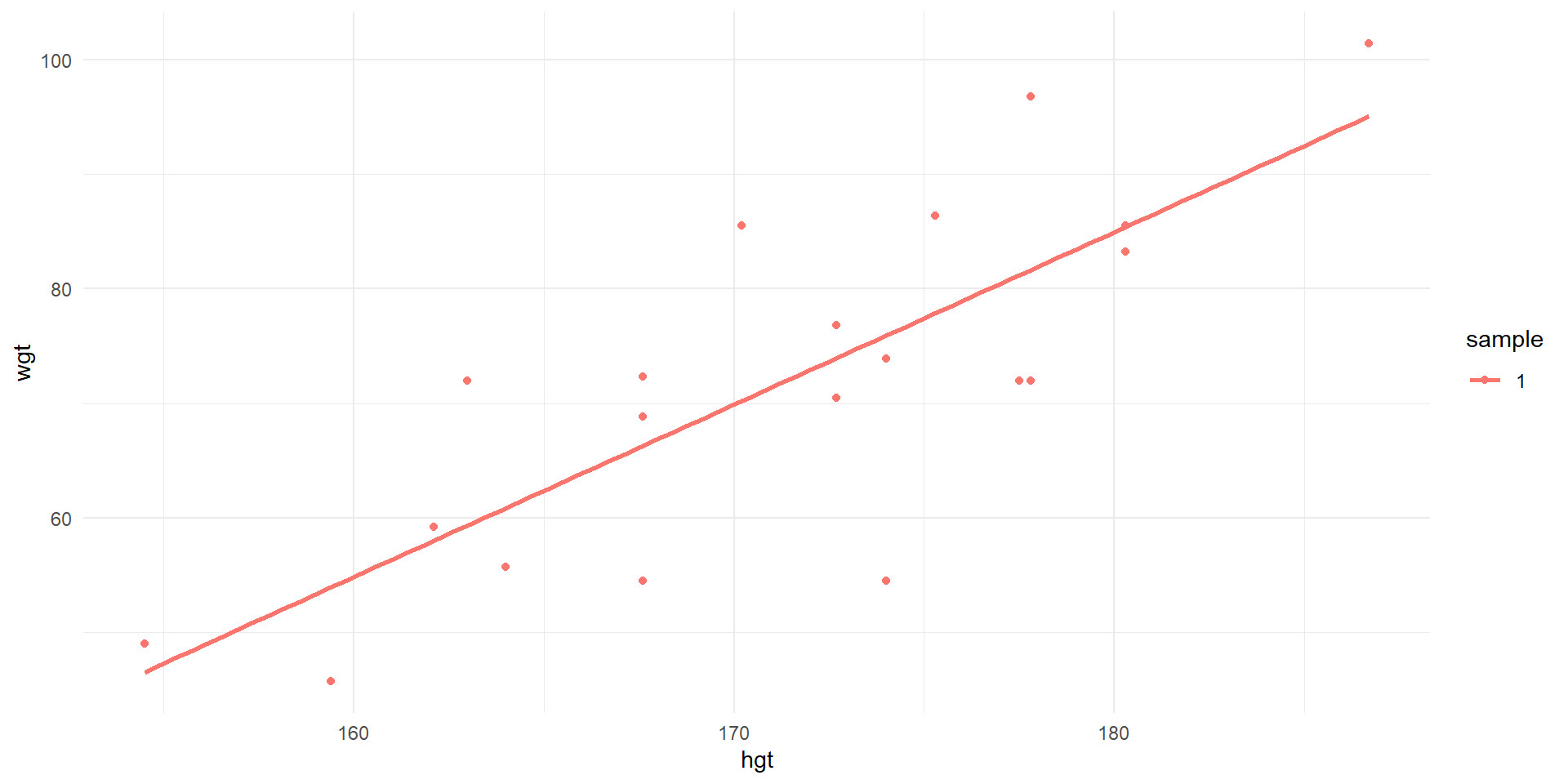
Observations of wgt vs. hgt and least squares line for first sample of 20.

Sample 1

term	estimate	std.error	statistic	p.value
(Intercept)	-186.302648	47.3081367	-3.938068	0.0009641
hgt	1.507037	0.2759548	5.461175	0.0000346

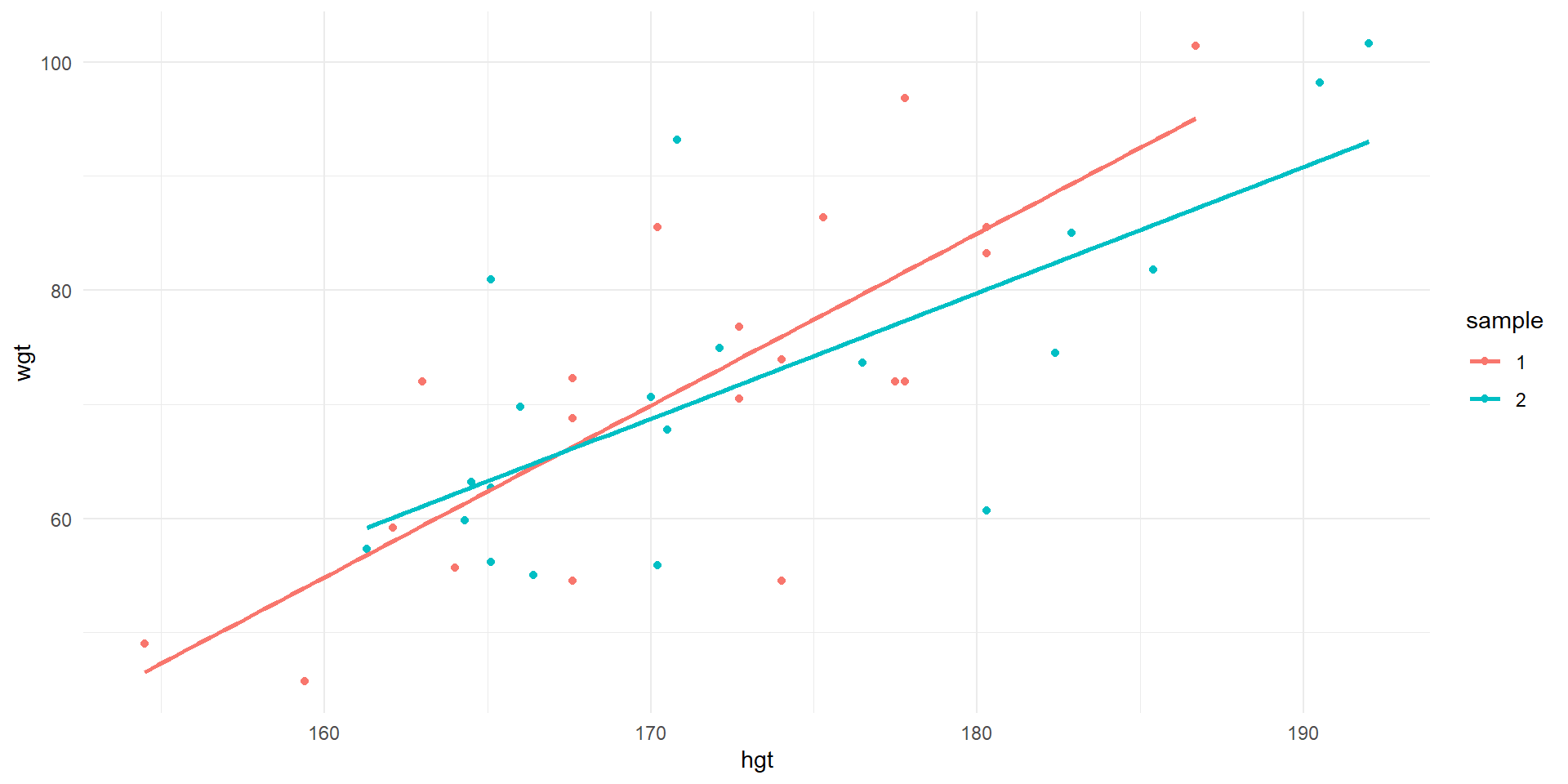
Observations of wgt vs. hgt and least squares lines for first two samples of 20.

Sample 2

term	estimate	std.error	statistic	p.value
(Intercept)	-186.302648	47.3081367	-3.938068	0.0009641
hgt	1.507037	0.2759548	5.461175	0.0000346

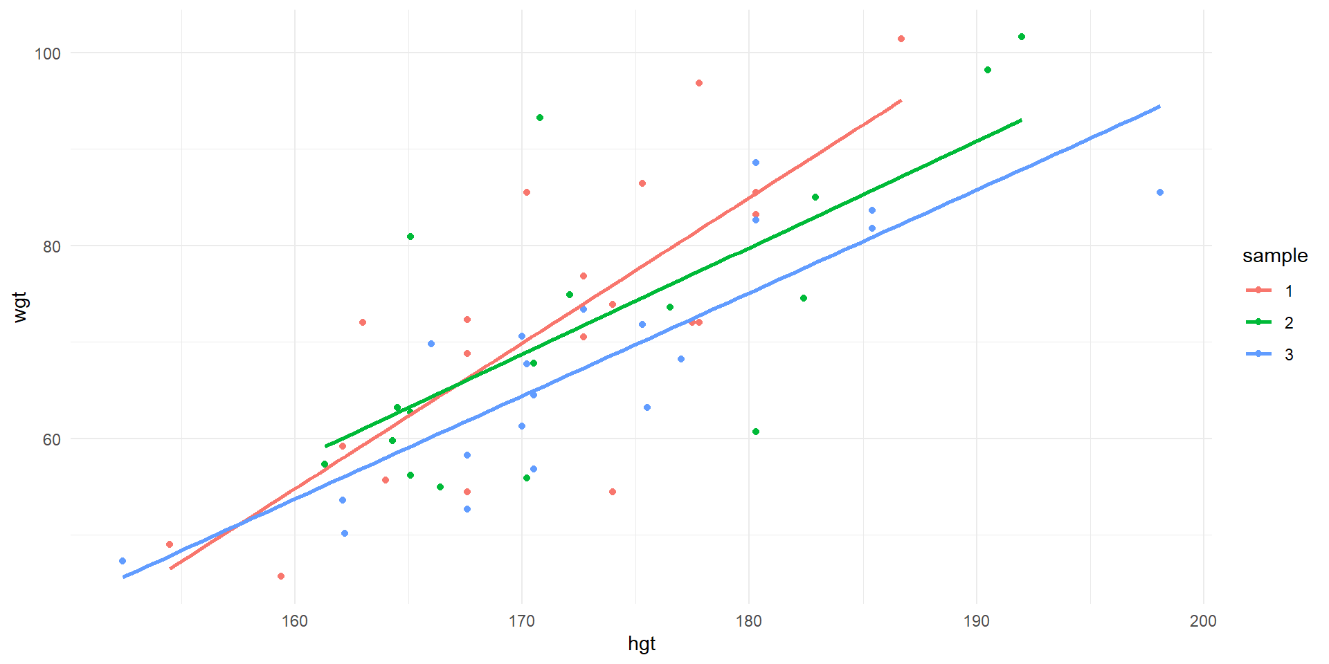
Observations of wgt vs. hgt and least squares lines for first three samples of 20.

Sample 3

term	estimate	std.error	statistic	p.value
(Intercept)	-186.302648	47.3081367	-3.938068	0.0009641
hgt	1.507037	0.2759548	5.461175	0.0000346

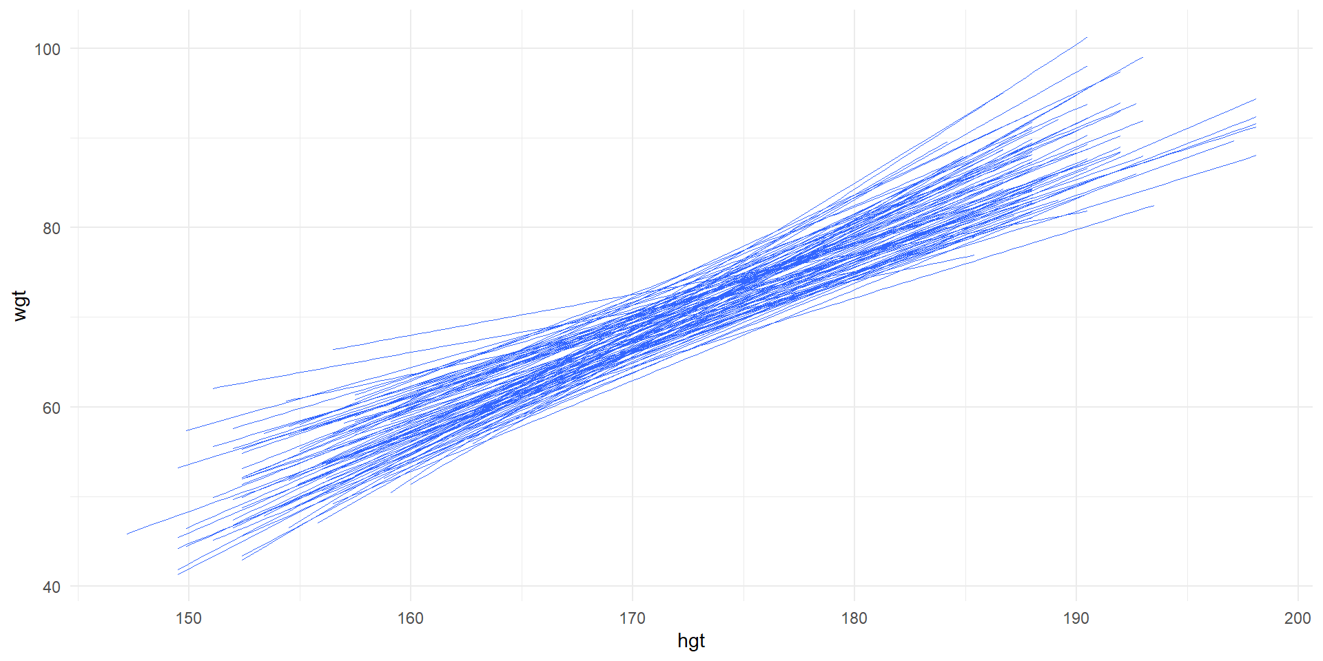
Least squares lines for 100 random samples of 20.

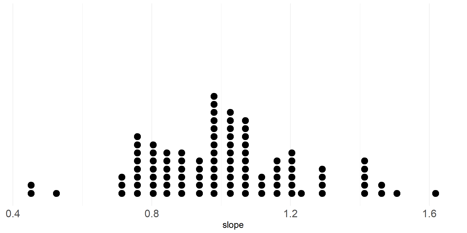
Dotplot of slopes of least squares lines from 100 random samples.

n	mean	sd
100	1.009732	0.220826

Inference for a Slope

Recall that a linear model with one predictor has the form \[\widehat{y}=b_0+b_1x\]
$b_0$ and $b_1$ are point estimates of the intercept and slope based on the sample (statistics)
$\beta_0$ and $\beta_1$ are the population intercept and slope (parameters)

We can conduct hypothesis tests for the slope
Typically, the null hypothesis is \[H_0:\beta_1=\beta_{1,0}\]
$\beta_{1,0}$ denotes the value of the slope under the null hypothesis
The null hypothesis that we will be focused on states that there is no association between the explanatory variable and the response variable
It would imply that the slope of the regression line is $0$: \[\boxed{H_0:\beta_1=0}\]
The alternative hypothesis could be one-sided or two-sided, depending on the research question

Hypothesis Test Using Randomization

Let us run a test to see if there significant evidence of the linear relationship between weight and height
Since the direction of the test is not indicated, we will use a two-sided alternative: \[H_0:\beta_1=0\] \[H_A:\beta_1 \ne 0\]
We can randomly permute the value of the response (wgt) to simulate the null hypothesis
Each time, compute the slope of the relationship between Wgt and hgt

Let us run 100 such simulations first

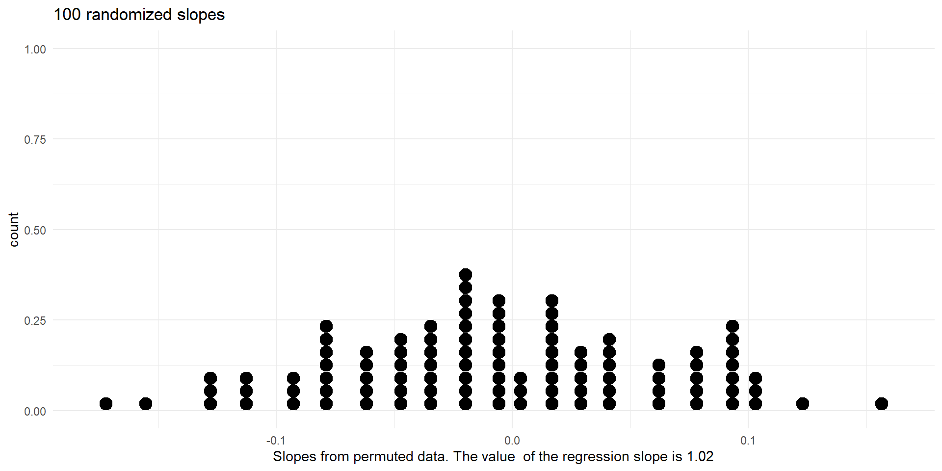
Now we will conduct 1,000 simulations

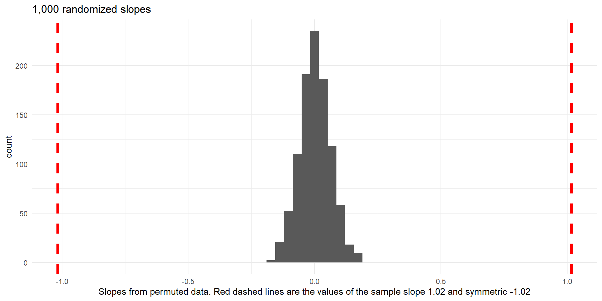
p-value $\approx0$

Test Statistic for Slope

The test statistic for a slope is is a $T$ statistic \[T=\frac{b_1-\beta_{1,0}}{SE}\]
$\beta_{1,0}$ denotes the value of the slope under the null hypothesis (usually 0)
The formula for the standard error for the slope is \[SE = \frac{s}{\sqrt{\sum_{i=1}^n(x_i-\bar{x})^2}}\]

$s$ estimates the standard deviation of the residuals, given by \[\begin{array}{rcl}s &=& \sqrt{\frac{SSE}{n-2}}\\ &=& \sqrt{\frac{\sum_{i=1}^n(y_i-\hat{y}_i)^2}{n-2}}\end{array}\]
Recall that $SSE$ is the sum of squared errors, also called the residual sum of squares ($RSS$)

Mathematical Model for Slope

Note

When the null hypothesis is true and the following conditions are met, the $T$ score has a $t$-distribution with $df=n-2$ degrees of freedom.

Linearity
Independent observations
Normality of residuals
Constant variability

One way to check conditions is to look at residual plots.

Checking Conditions

Linearity? Independent observations? Normality of residuals? Constant variability?

Technical conditions are approximately satisfied
- Scatterplot appears to be approximately linear
- Observations appear to be independent
- Residuals approximately normal and have approximately constant variability
The results of the test are in the line that is labeled by the explanatory variable (hgt)
The value of the T-score ($T=23.1$) and the corresponding p-value of the two-sided test are given in the regression table

term	estimate	std.error	statistic	p.value
(Intercept)	-105.011254	7.5394092	-13.92831	0
hgt	1.017617	0.0439868	23.13459	0

Note that the regression table always provide p-values for two-sided tests

CI Using Randomization

We can also calculate a 95% bootstrap percentile confidence interval based on the entire sample
We will create bootstrapped samples and calculate resulting slopes of the regression lines
Then we will create the distribution of the bootstrapped slopes

Let us create 100 bootstrapped slopes first

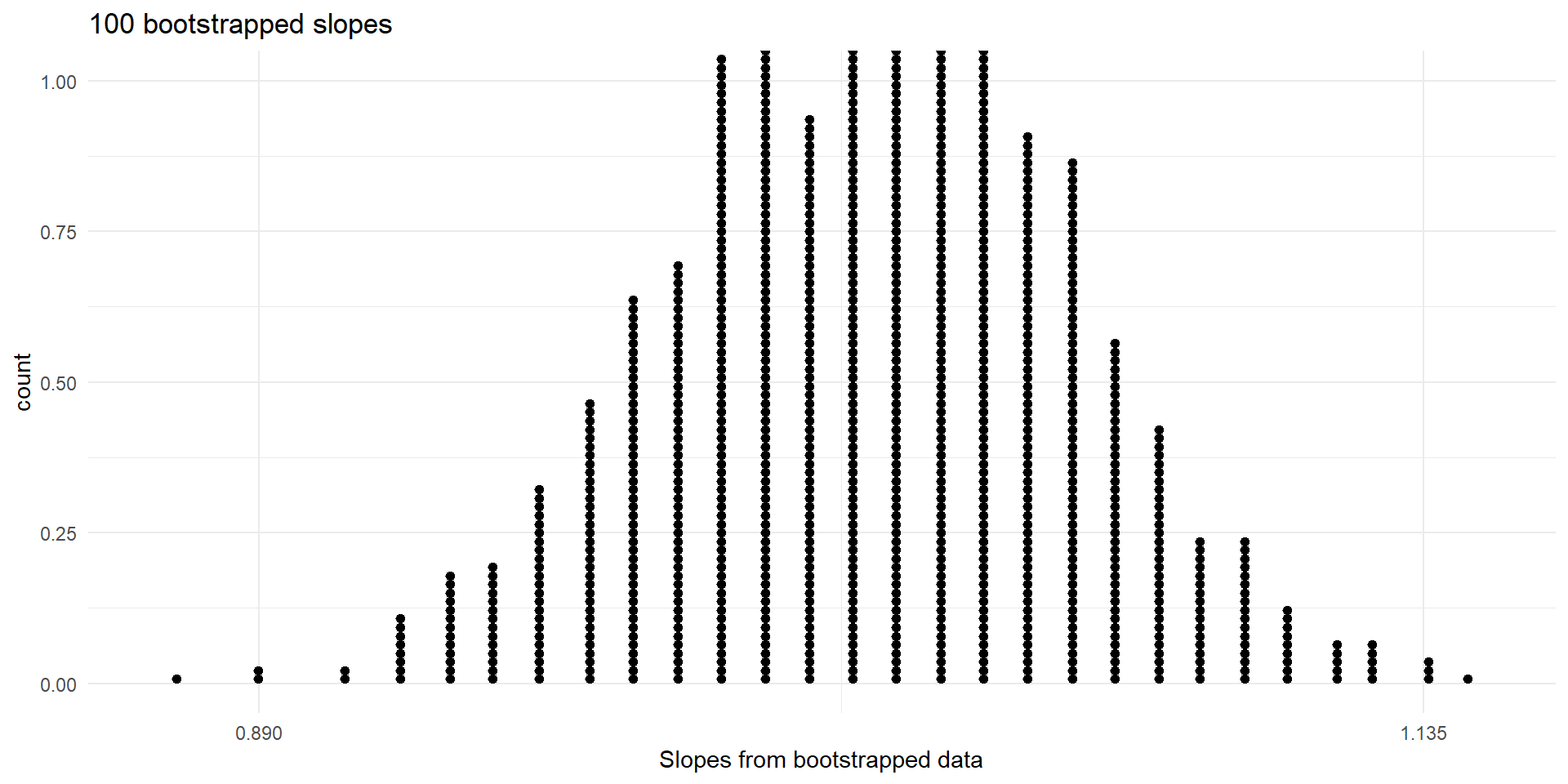
Now we will use 1,000 bootstrapped slopes

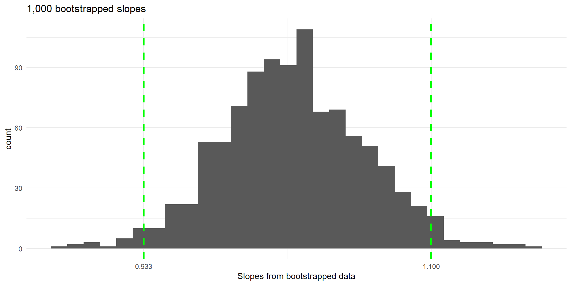
95% bootstrap percentile confidence interval: $(0.933, 1.10)$
We are 95% confident that the slope is between 0.933 and 1.10, meaning that the weight increases from 0.933 to 1.1 kilograms for each increase of 1 cm in the height.

Confidence Interval using Mathematical Model

If the technical conditions are met we can also use a $t$ distribution with $df=n-2$ to calculate a confidence interval for the slope
The interval is \[b_1\pm t^{\ast}_{df}\times SE\]
The standard error is the same as we used for the hypothesis test (from regression table $SSE=0.044$)

term	estimate	std.error	statistic	p.value
(Intercept)	-105.011254	7.5394092	-13.92831	0
hgt	1.017617	0.0439868	23.13459	0

The value of $t^{\ast}_{df}$ depends on the confidence level and degrees of freedom
For example, for a 95% confidence itreval will be $t^{\ast}_{505}=1.965$
Finally, 95% confidence interval for the slope of the regression line will be \[1.02 \pm 1.965 \cdot 0.044=(0.934,1.106)\]

Conclusions

There is convincing evidence that there is an association between weight and height (p-value < 0.001)
We are 95% confident that the weight increases from 0.933 to 1.1 kilograms for each increase of 1 cm in the height.
We can generalize the results to a larger population since it is a random sample
This is an observational study, so we cannot conclude a cause-and-effect relationship between the variables
Note that the confidence interval is consistent with the test since we rejected value 0

Italian Restaurants in NYC

Is the price of a meal associated with food quality?
restNYC dataset¹ is available here
Customer survey from Italian restaurants in NYC ($n$ = 168)
Price (USD, includes tip and drink)
Food (rating: 1 to 30)

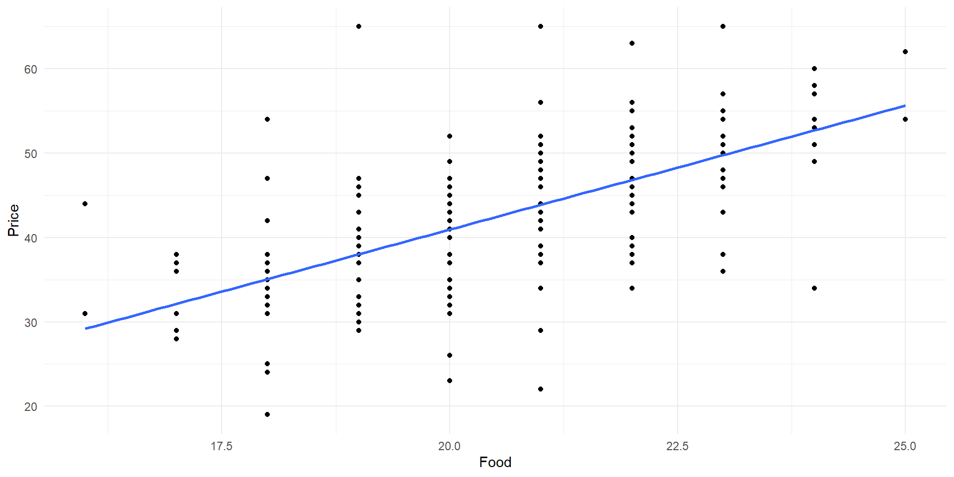
Scatter plot of Price vs Food with least squares line.

Fitting a Linear Model

Least squares regression line \[\widehat{Price}=-17.8+2.94\times Food\]
Recall that we can use Jamovi to find the equation for the regression line (see, e.g., J Lab 4)

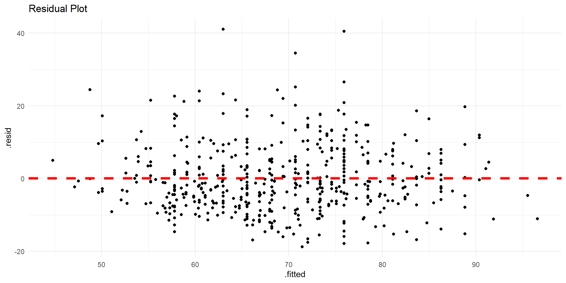
Checking Conditions

Linearity? Independent observations? Normality of residuals? Constant variability?

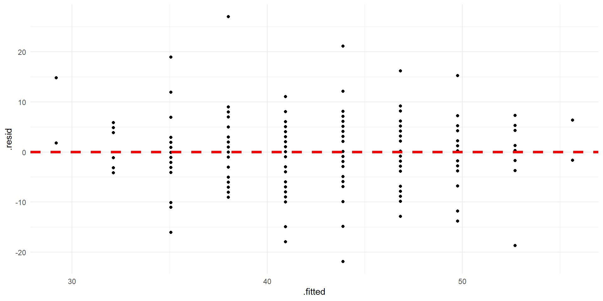
Residual plot.

Hypothesis Test Using Mathematical Model

Hypothesis test: \[H_0: \beta_1=0, H_A: \beta_1\neq0\]

term	estimate	std.error	statistic	p.value
(Intercept)	-17.83215	5.8631197	-3.04141	0.0027375
Food	2.93896	0.2833809	10.37106	0.0000000

$T$ = 10.4
$df = 168-2=166$
p-value < 0.001

Hypothesis Test Using Randomization

We can randomly permute the value of the response (Price) to simulate the null hypothesis
Each time, compute the slope of the relationship between Price and Food

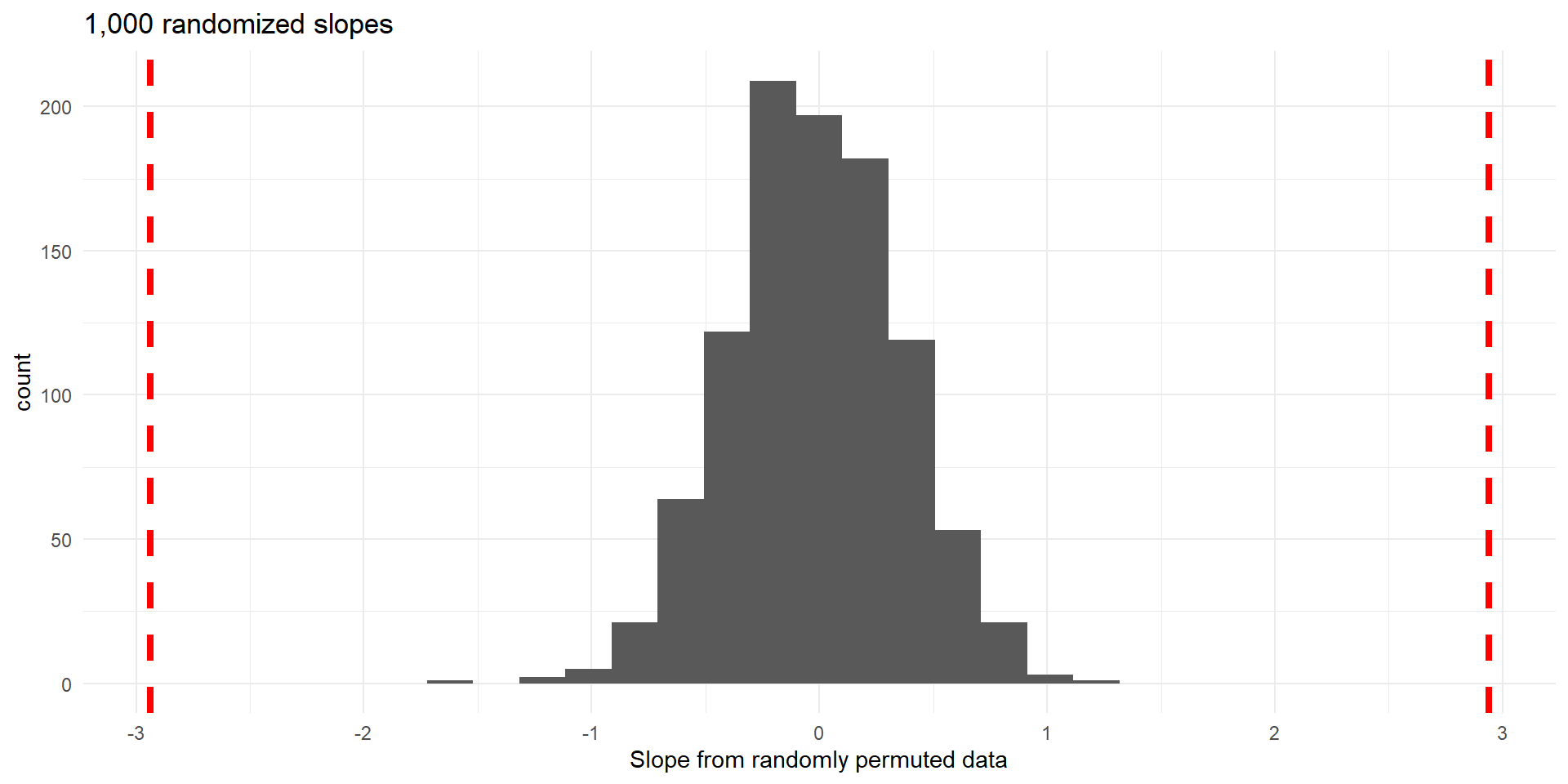
Histogram of slopes from different random permultations of Price (null distribution).

The proportion of values $\ge 2.94$ or $\le -2.94$ is 0, so p-value $\approx0$

CI Using Randomization

We can also calculate a 95% bootstrap percentile confidence interval

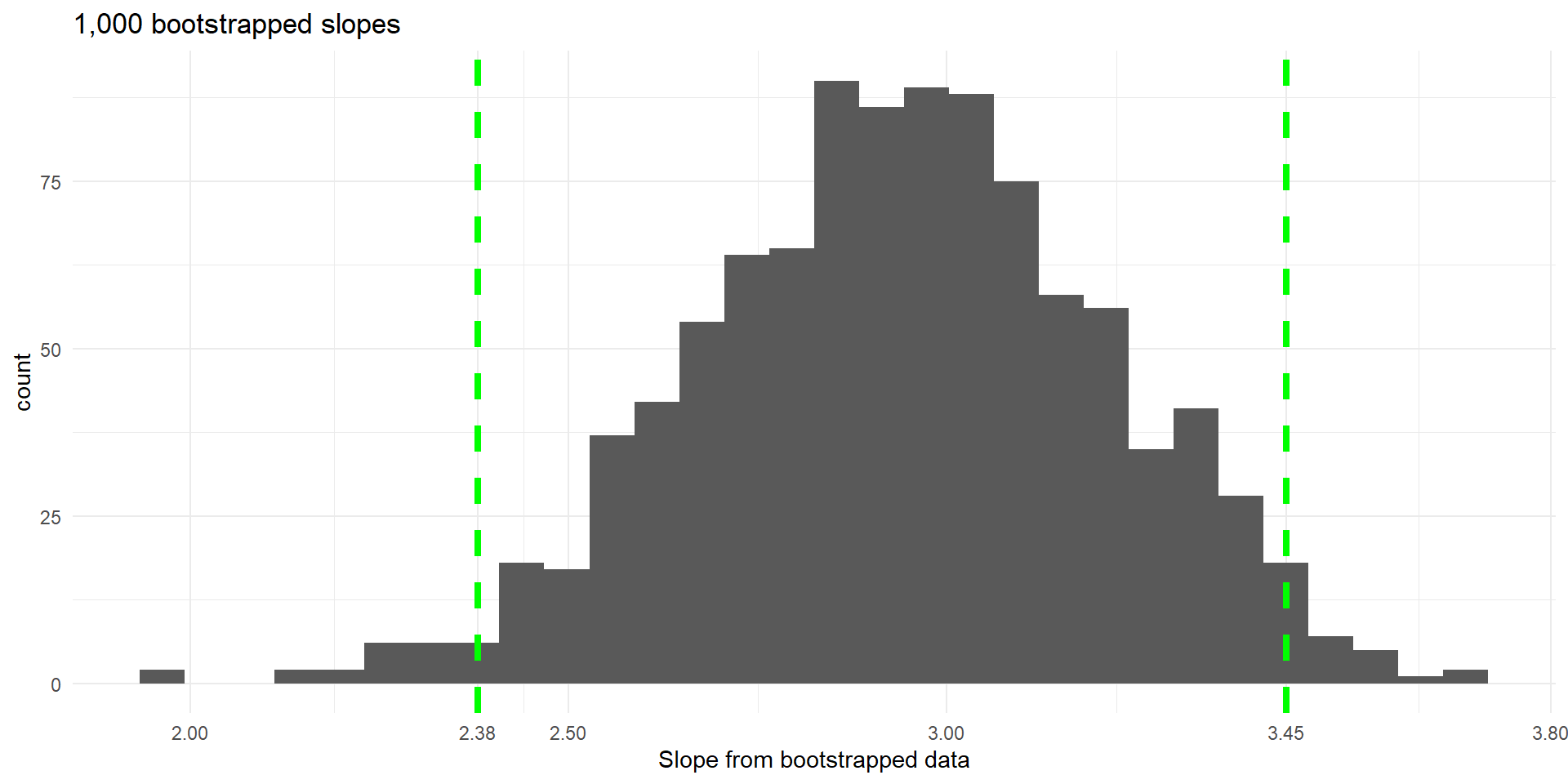
Histogram of slopes from bootstrapped data.

95% bootstrap percentile confidence interval: (2.38, 3.45)

rest_boot |>
  get_confidence_interval(level = 0.95, type = "percentile")

We are 95% confident that the slope is between 2.38 and 3.45, meaning that the price of a meal increases by between $2.38 and $3.45 for each increase of 1 point in the food rating.

CI Using Mathematical Model

A 95% confidence interval for the slope is given by \[b_1\pm t^{\ast}_{df}\times SE\]
$SE=0.283$ (from regression output)

term	estimate	std.error	statistic	p.value
(Intercept)	-17.83215	5.8631197	-3.04141	0.0027375
Food	2.93896	0.2833809	10.37106	0.0000000

Since, $df = 166$, $t^{\ast}_{df}=1.974$ for a 95% CI
The 95% CI is $2.94\pm1.974\times0.283=(2.34, 3.49)$.

Conclusions

There is convincing evidence that there is an association between price and food rating in NYC Italian restaurants (p-value < 0.001)
We are 95% confident that the price increases from $2.34 to $3.49 per 1 unit increase in ratings
We do not know if this is a random sample, so we should be careful about generalizing the results
This is an observational study, so we cannot conclude a cause-and-effect relationship between the variables