Compare Paired Means

Chapter 21
Math 115

What would you do?

  • How would you go about collecting your data for each of the following?
    • You want to compare grocery prices between Meijer and Family Fare. Are prices different, on average?
    • You want to test “The Freshmen 15” theory. Do college students gain, on average, 15 pounds during their first year?
  • The paired datasets in this chapter have one pair of quantitative response values for each observational unit.
  • This allows for a built-in comparison.
  • Studies with paired data remove individual variability by looking at the difference score for each individual.
  • Reducing variability in data improves inferences:
    • Narrower confidence intervals
    • Smaller p-values when the null hypothesis is false

Studying with Music

  • Many students study while listening to music.
  • Does it hurt their ability to focus?
  • In “Checking It Out: Does music interfere with studying?” Stanford Prof Clifford Nass claims the human brain listens to song lyrics with the same part that does word processing
  • Instrumental music is, for the most part, processed on the other side of the brain and Nass claims that reading and listening to instrumental music has virtually no interference.

Experimental designs:

  • Experiment 1—Random assignment to 2 groups (Independent groups)
    • 27 students were randomly assigned to 1 of 2 groups:
    • One group listens to music with lyrics
    • One group listens to music without lyrics
    • Students play a memorization game while listening to the particular music that they were assigned.
  • Experiment 2—Paired design using repeated measures
    • All students play the memorization game twice (randomly assigning the order):
    • Once while listening to music with lyrics
    • Once while listening to music without lyrics.
  • Experiment 3—Paired design using matching
    • Test each student on memorization.
    • Match students up with similar scores and randomly:
    • Have one play the game while listening to music with lyrics and the other while listening to music without lyrics.
  • What if everyone could remember exactly 2 more words when they listened to a song without lyrics?
  • There could be a lot of overlap between the two sets of scores and it would be difficult to detect a difference as shown here.
  • We need to focus on differences within matching pairs

Textbook prices

  • Will you save money if you buy textbooks from Amazon instead of a university bookstore?
  • We will compare prices of books from Amazon and the UCLA bookstore
  • For each book in the data we will calculate the difference between the book’s price at the UCLA bookstore and its price on Amazon
  • Since our data consists of a single difference for each book, the analysis will be similar to the single mean case

Data

  • ucla_textbooks_f18 1 dataset available here
  • Sample of 68 books used in courses at UCLA in 2018
  • bookstore_new is price of new book at bookstore
  • amazon_new is price of new book on Amazon
ucla_textbooks_f18
# A tibble: 68 × 4
   subject                 course_num bookstore_new amazon_new
   <fct>                   <fct>              <dbl>      <dbl>
 1 American Indian Studies M10                48.0       47.4 
 2 Anthropology            2                  14.3       13.6 
 3 Arts and Architecture   10                 13.5       12.5 
 4 Asian                   M60W               49.3       55.0 
 5 Astronomy               4                 120.       125.  
 6 Communication           10                 17.0       11.8 
 7 Comparative Literature  2CW                12.0       10.9 
 8 Dance                   10                 26.8       38.9 
 9 English                 19                  9.96       8.99
10 English Composition     1A                 40.0       35   
# ℹ 58 more rows

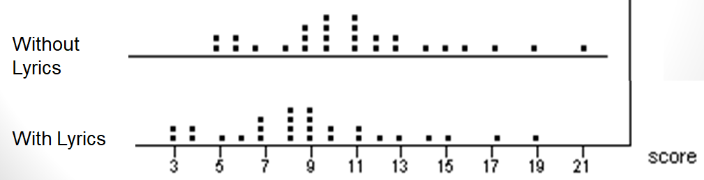
Here are side-by-side dotplots

  • One way to analyze the data would be to treat the books on Amazon and the books at the bookstore as two groups. Then we could compare the difference in the group means as we did in Chapter 20
  • Each observation would be a book on Amazon or a book at the bookstore
  • However, this ignores the paired structure of the data (observations are not independent)
  • Such analysis would not use all available information and will have lower power

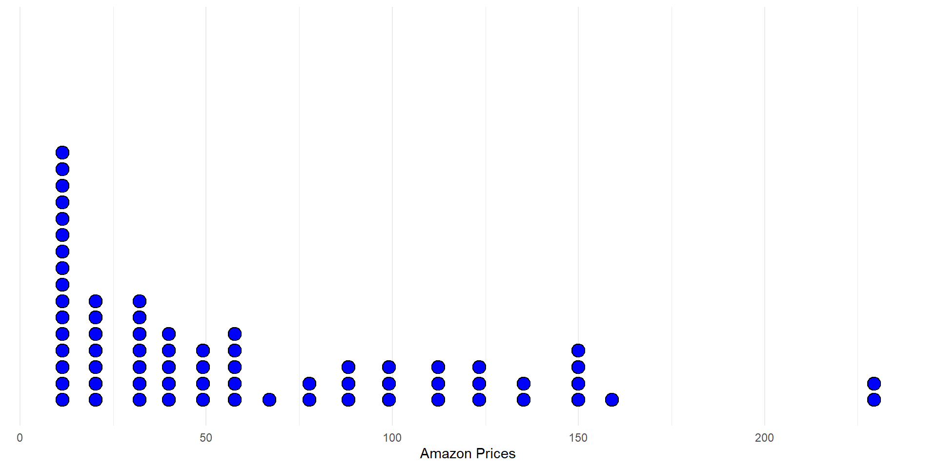
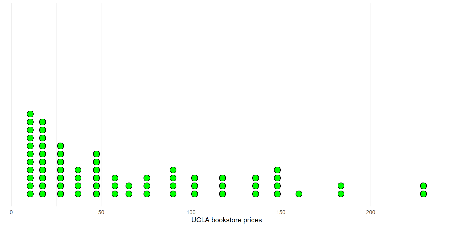
Paired dotplots and histogram of differences

ucla_textbooks_f18 <- ucla_textbooks_f18 |>
  mutate(price_diff = bookstore_new - amazon_new)

ucla_textbooks_f18
# A tibble: 68 × 5
   subject                 course_num bookstore_new amazon_new price_diff
   <fct>                   <fct>              <dbl>      <dbl>      <dbl>
 1 American Indian Studies M10                48.0       47.4       0.520
 2 Anthropology            2                  14.3       13.6       0.710
 3 Arts and Architecture   10                 13.5       12.5       0.97 
 4 Asian                   M60W               49.3       55.0      -5.69 
 5 Astronomy               4                 120.       125.       -4.83 
 6 Communication           10                 17.0       11.8       5.18 
 7 Comparative Literature  2CW                12.0       10.9       1.09 
 8 Dance                   10                 26.8       38.9     -12.2  
 9 English                 19                  9.96       8.99      0.97 
10 English Composition     1A                 40.0       35         4.97 
# ℹ 58 more rows
  • By analyzing the difference in price, we account for the paired structure
  • Each observation is a different book

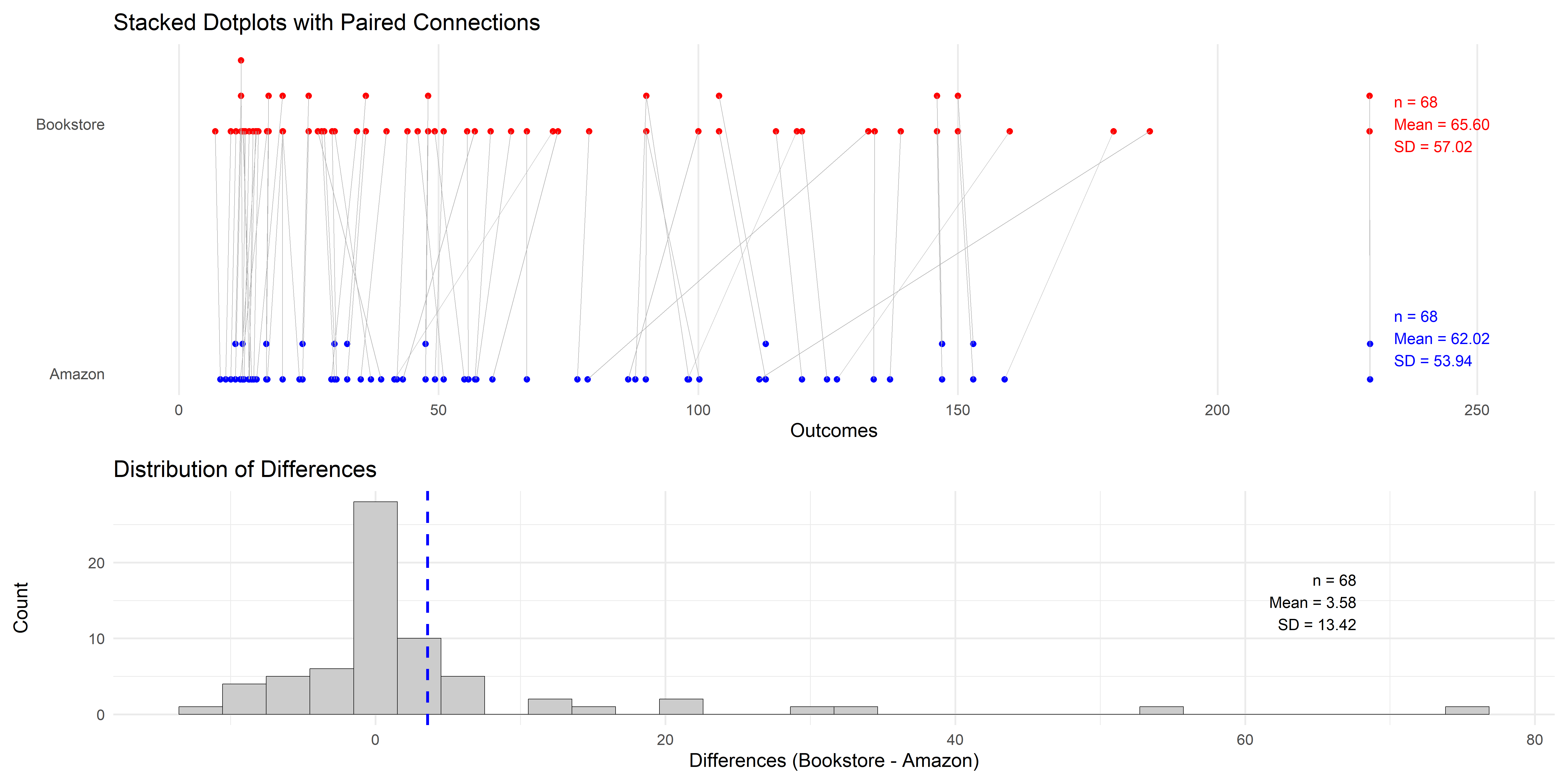
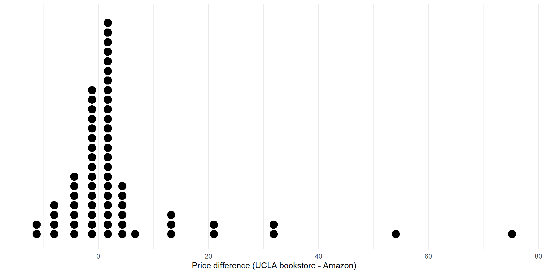
Differences in prices

Price differences (USD) between UCLA bookstore and Amazon for 68 books.
n mean median sd iqr
68 3.58 0.625 13.4 3.98
  • The observed mean difference is \(\bar{x}_{diff}=3.58\)
  • Based on the shape of the distribution, you could easily argue that the median is a more appropriate measure of center!
  • However, since the sample size is greater than 30, the means will have approximately t-distribution

Inference

  • We will estimate the difference mean difference in book price \(\mu_{diff}\) using a confidence interval
  • We will conduct a hypothesis test with hypotheses
    • \(H_0: \mu_{diff} = 0\)
    • \(H_A: \mu_{diff} \neq 0\)
  • We will calculate differences with the order (UCLA - Amazon)

Hypothesis Test Using Random Permutation

  • We can use randomization to simulate variability in the statistic under a true null hypothesis
  • To simulate independence between price and bookseller, we randomly reassign the book prices for each book
  • E.g., here are the data for the first book
subject course_num bookstore_new amazon_new price_diff
American Indian Studies M10 \(\color{blue}{47.97}\) \(\color{green}{47.45}\) 0.52
  • Random reassignment results in one of two possible outcomes: original prices or swapped prices
subject course_num bookstore_new amazon_new price_diff
American Indian Studies M10 \(\color{blue}{47.97}\) \(\color{green}{47.45}\) 0.52

Or

subject course_num bookstore_new amazon_new price_diff
American Indian Studies M10 \(\color{green}{47.97}\) \(\color{blue}{47.45}\) -0.52
  • We can think of the randomization as flipping a coin for each book to determine which of the two assignments will occur in the randomized sample
  • Let’s create 1,000 random permutations of the data

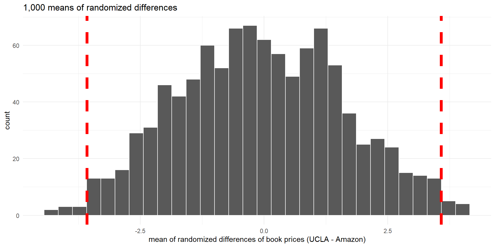
Histogram of 1,000 mean of randomized differences (null distribution). Dashed vertical lines indicate differences of 3.58 (observed mean difference) and -3.58.

  • The p-value is the proportion of the means of differences that are at least as extreme as the observed mean difference (3.58)

  • In this histogram there are 17 outcomes that are as extreme as the value \(\bar{x}_{diff}= 3.58\), so p-value is 0.017

  • We reject the null hypothesis, and conclude that Amazon prices are, on average, different from UCLA bookstore prices

  • In fact, UCLA bookstore prices are higher than Amazon prices

Conclusion

  • Let’s summarize our findings in a full conclusion
    • We reject the null hypothesis, and conclude that Amazon prices are, on average, different from UCLA bookstore prices
    • In fact, UCLA bookstore prices are higher than Amazon prices
    • We cannot generalize these results to a larger population since it was not a random sample
    • We cannot draw cause-and-effect conclusion since it was an observational study

Boostrap Confidence Intervals

  • We can calculate bootstrap confidence intervals (percentile or SE) using the same approach as in the singe mean case
  • We resample the price differences (UCLA - Amazon) from the sample with replacement to simulate the variablility in the statistic
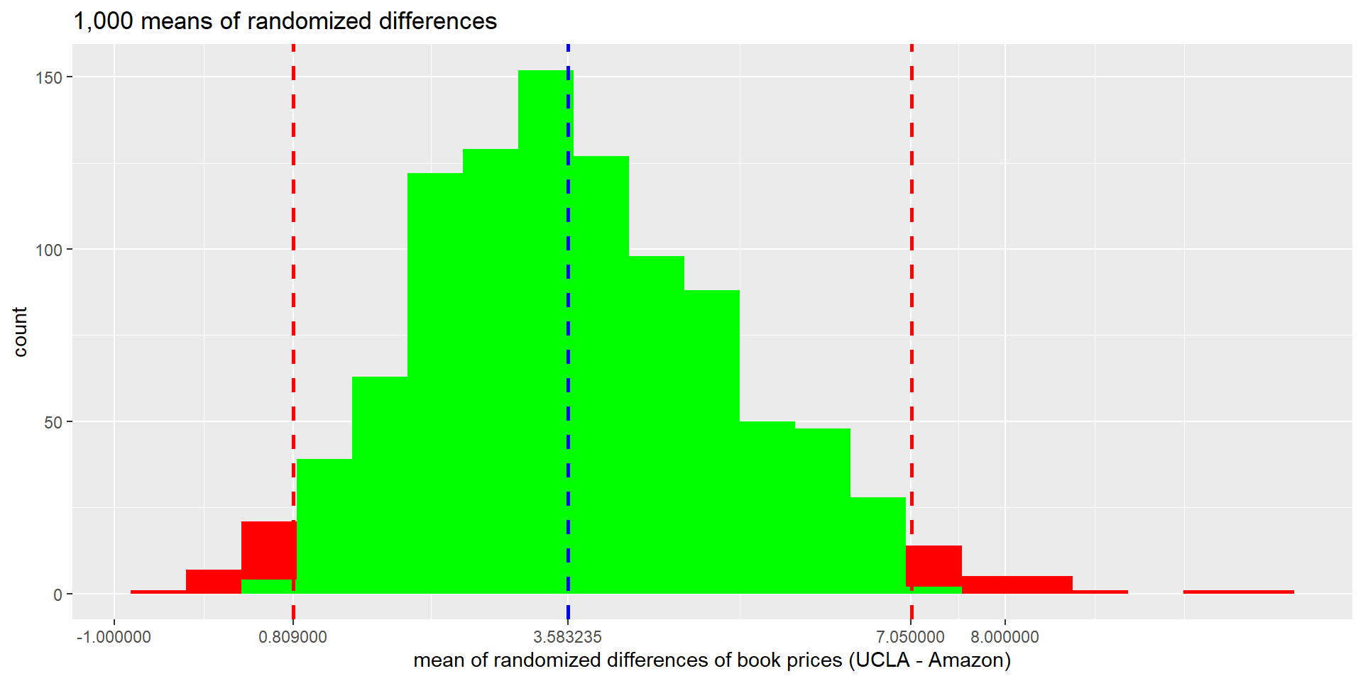
  • The 95% bootstrap percentile confidence interval for the mean price difference is \((\$0.809, \$7.05)\).
  • We can also use the standard error (\(SE\)) of the bootstrap distribution to find the confidence interval
  • \(SE=1.63\)
  • The 95% bootstrap SE confidence interval is \(3.58\pm1.96\times1.63\)
  • So the bounds are ($0.385, $7.77)

Hypothesis Test Using a Mathematical Model

  • We can use the same mathematical model as the single mean case to conduct a hypothesis test
  • The standard error for the mean difference is \[SE_{diff}=\frac{s_{diff}}{\sqrt{n_{diff}}}=\frac{13.4}{\sqrt{68}}=1.62\]
  • The \(T\) statistic is \[T=\frac{\bar{x}_{diff}-0}{SE_{diff}}=\frac{3.58-0}{1.63}=2.20\]
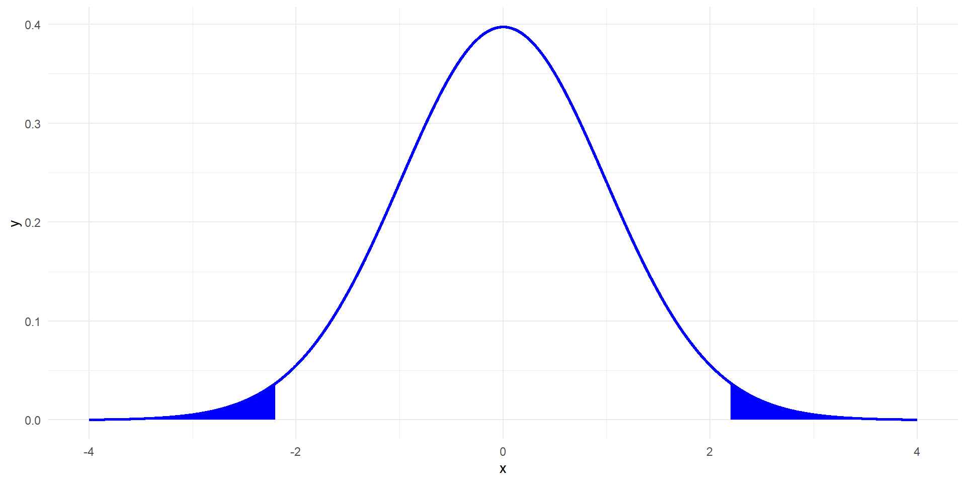
  • The degrees of freedom are \(df = 68-1=67\)

  • We can calculate a p-value by finding the area in the two tails of the \(t\)-distribution with \(df=67\) that is beyond -2.20 or 2.20

  • p-value of the two-sided test is 0.031

  • We can also find it in Jamovi

Confidence Interval Using a Mathematical Model

  • We can also use a mathematical model to calculate confidence intervals

  • The interval is \[\bar{x}_{diff}\pm t^{\ast}_{df}\times SE_{diff}\]

  • For a 95% CI, \(t^{\ast}_{67}=1.996\)

  • A 95% CI is given by \(3.58\pm1.996×1.62=(\$0.346, \$6.81)\)

  • We are 95% confident that the long-run average difference in bookstore prices (UCLA bookstore price - Amazon price) is between \(\$0.346\) and \(\$6.81\)
  • In other words, UCLA bookstore prices are from \(\$0.346\) to \(\$6.81\) dollars higher than Amazon prices
  • This CI is consistent with the result of the test of significance since value 0 (value of the null hypothesis) is not in the confidence interval