Compare Two Independent Means
Chapter 20
Math 219
Math 219
Birth Weights and Smoking
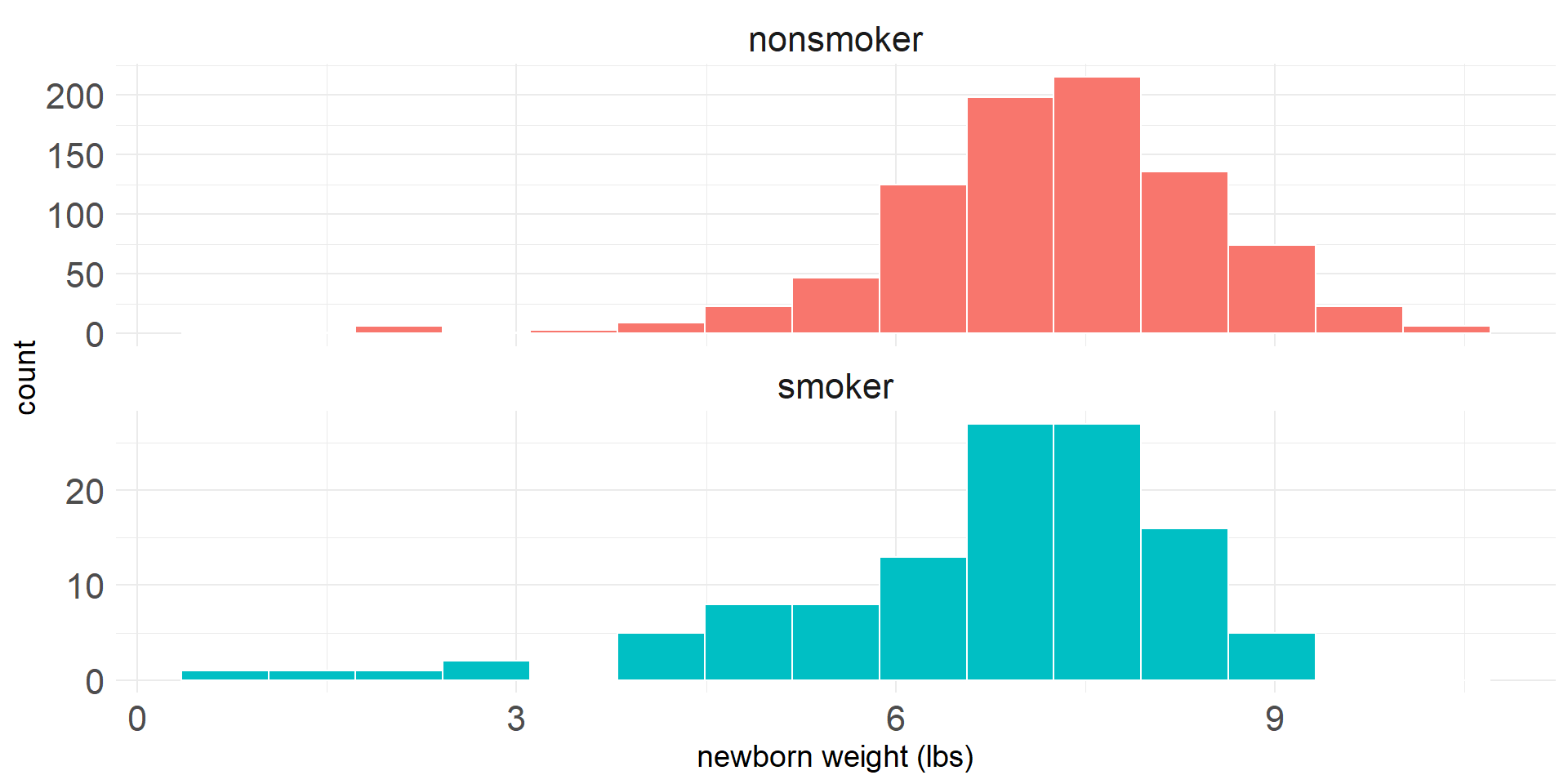
- Do infants whose mothers do not smoke have higher mean birth weight than infants whose mothers do smoke?
- Let \(\mu_n\) be the population’s mean weight (lbs) of infants whose mothers did not smoke, and let \(\mu_s\) be the population’s mean for infants whose mothers smoked
- Note, as always we difine the parameters of populations
Inference
- We will conduct a hypothesis test with hypotheses
- \(H_0: \mu_n-\mu_s = 0\)
- \(H_A: \mu_n-\mu_s \ne 0\)
- We can also state these hypotheses in therm of association:
- \(H_0:\) There is no association between birth weight and smoking status
- \(H_A:\) There is an association between birth weight and smoking status
Data
births14dataset available here- Random sample of 1,000 cases from US birth data set from 2014 (19 removed with missing values)
habitis smoking habit (“smoker” or nonsmoker”)weightis birth weight in pounds
EDA
| habit | n | mean | sd |
|---|---|---|---|
| nonsmoker | 867 | 7.27 | 1.23 |
| smoker | 114 | 6.68 | 1.60 |
The test statistic will be the observed difference in means is \[\boxed{\begin{array}{lcr}\bar{x}_n-\bar{x}_s &=& 7.27-6.68\\ &=& 0.59\end{array}}\]
Randomization Test for Difference in Means
- We can simulate a true null hypothesis by randomly permuting the values of the response variable
- This similar to what we did in Chapter 11 and then in Chapter 17
- The main difference is that our response variable is quantitative
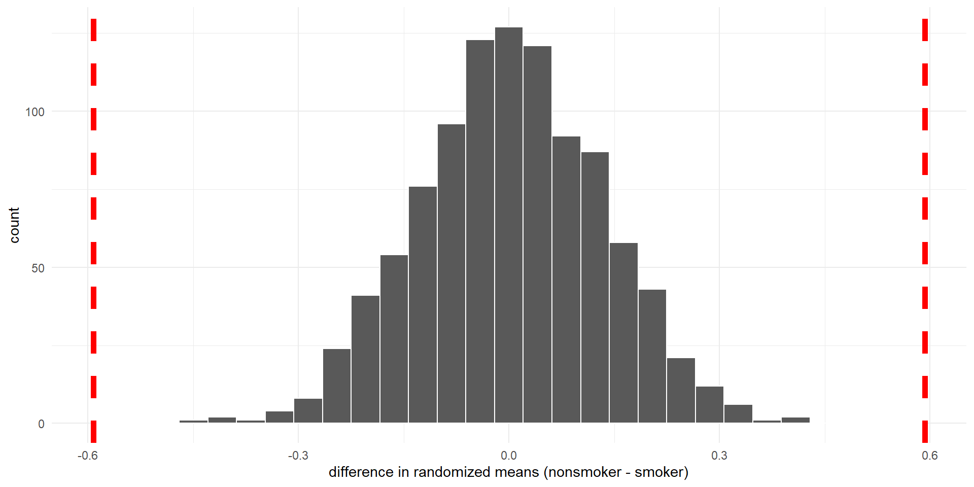
Histogram of differences in means (null distribution) calculated from 1,000 random permutations of birth weights. Observed difference is 0.59.
- The p-value is the proportion of randomized differences that are at least as extreme as the observed value (\(\geq\) 0.59 or \(\leq\) -0.59)
- There are no such randomized differences, so the p-value is approximately 0
Test Statistic for Comparing Two Means
- The test statistic for comparing two means is the \(T\) statistic (\(T\) score)
- We will use a version of the \(T\) statistic that assumes the two populations have equal variance (different than the version presented in the text)
Pooled Sample Standard Deviation
First we compute the pooled sample standard deviation, \[s_p = \sqrt{\frac{(n_1-1)s_1^2+(n_2-1)s_2^2}{n_1+n_2-2}}\]
The pooled sample standard deviation in birth weights is \[\begin{array}{rcl} s_p &=& \sqrt{\frac{(867-1)\cdot 1.23^2+(114-1)\cdot 1.60^2}{867+114-2}}\\ &=& 1.28\end{array}\]
The \(T\) statistic is \[T=\frac{(\bar{x}_1-\bar{x}_2)-0}{s_p\sqrt{\frac{1}{n_1}+\frac{1}{n_2}}}\]
For the birth weight example, the value is \[T=\frac{0.59-0}{1.28\cdot\sqrt{\frac{1}{867}+\frac{1}{114}}} = 4.63\]
Mathematical Model for Testing the Difference in Means
Note
When the null hypothesis is true and the following conditions are met, the \(T\) score has a \(t\)-distribution with \(df=n_1+n_2-2\) degrees of freedom.
- Groups have equal variance in the population
- Independent observations within and between groups
- Normality: Large samples and no extreme outliers.
Two Sample T-Test
- The degrees of freedom for the birth weight example is \(df=867+114-2=979\).
- We can use the Randomize module in Jamovi to calculate a p-value using a T distribution with 979 degrees of freedom
- Find the area that is above 4.63 (the observed value of \(T\)) or below -4.63
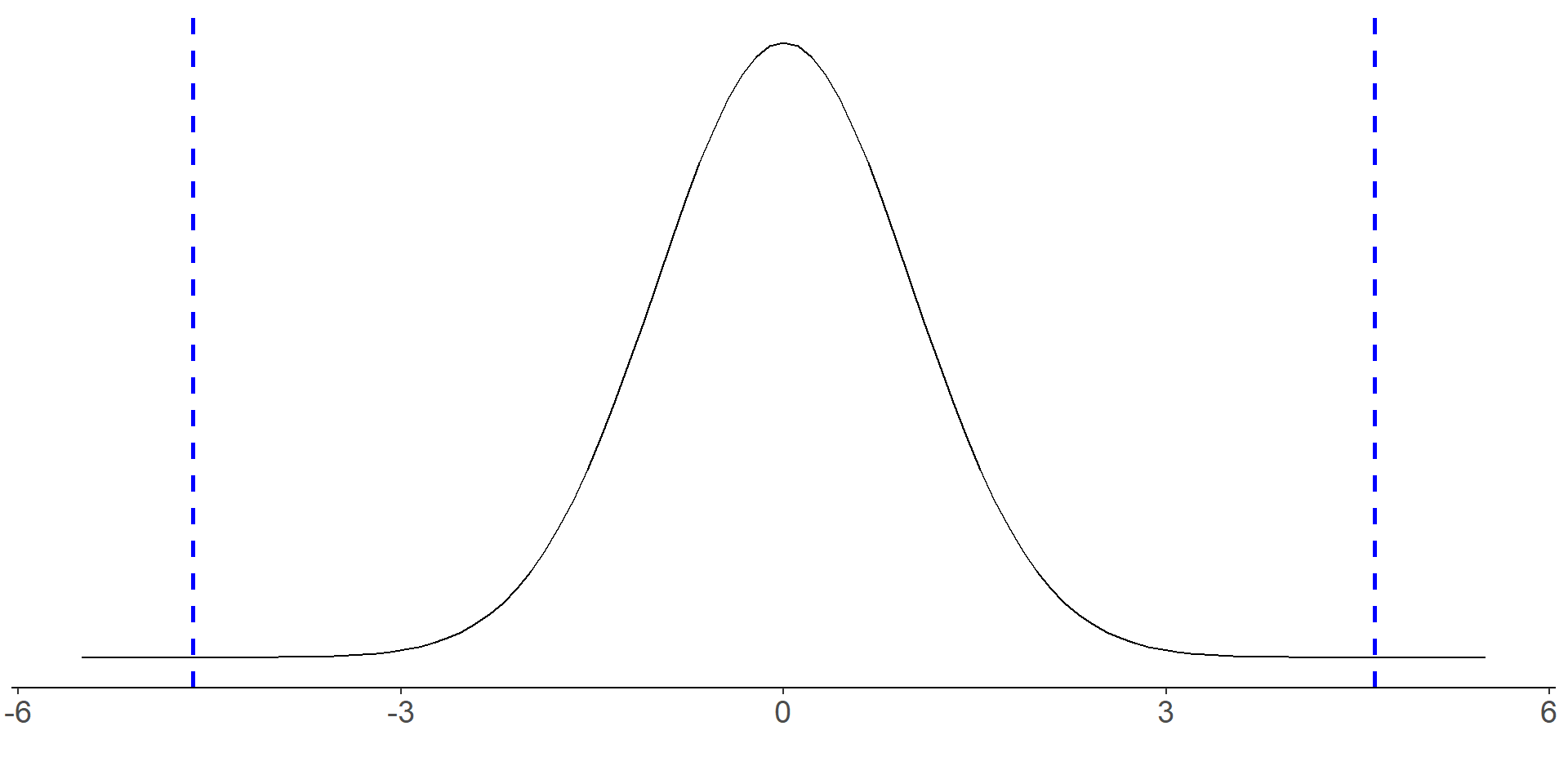
The \(t\)-distribution with 979 degrees of freedom. The observed \(T\)-statistic is 4.63. The p-value is the total area to the left of -4.63 or to the right of 4.63.
- The p-value is extremely small, p-value < 0.001
Bootstrap Confidence Interval for Difference in Means
- The method for calculating bootsrap confidence intervals for a difference in means is similar to the methods we used for a difference in proportions
- We create bootstrap samples from each group (resampling with replacement) and calculate a difference in means
- We do this 1,000 time and use the resulting sampling distribution to calculate a bootstrap percentile CI or a boostrap SE CI
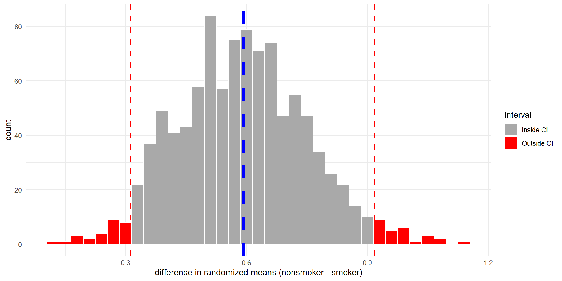
- Lets calculate differences in bootstrapped means for the birth weight example
- The 95% boostrap percentile CI is (0.312, 0.917)
Estimating the Difference in Means Using a Mathematical Model
If the technical conditions are met, including the equal variance assumption, then we can use the \(t\)-distribution to estimate the difference in means
We can calculate a confidence interval for the difference in means as \[(\bar{x}_1-\bar{x}_2)\pm t^{\ast}_{df}\times SE\]
Note that the value of standard errot (\(SE\)) is the same as in the formula for the T-score
- Assuming equal variance, \(df=n_1+n_2-2\), and the standard error is \[SE = s_p\sqrt{\frac{1}{n_1}+\frac{1}{n_2}}=0.128\]
- The value of \(t^{\ast}_{df}\) depends on the degrees of freedom and the confidence level
- Since \(df=979\) for this example, the value of \(t^{\ast}_{df}\) for a 95% confidence interval is 1.96
- Thus, the 95% confidence interval is \[0.59\pm1.96\times0.128=0.59\pm0.251\]
- In interval form it is approximately (0.339, 0.841)
Conclusions
- We reject the null hypothesis at the \(\alpha=0.05\) significance level and conclude that there is strong evidence that the average weights of infants born to mothers who did not smoke is different (in fact, it is higher) than the average weights of infants born to mothers who smoked (p < 0.001)
- We can generalize to a larger population since it was a random sample
- We cannot draw cause and effect conclusion since it was an observational study
- We are 95% confident that the mean weight of babies born to mothers who did not smoke is between 0.285 and 0.900 pounds higher than the mean weight of babies whose mothers smoked
- This result is also consistent with the result of the hypothesis test, since 0 does not appear in the 95% confidence interval
Note About Relaxing the Equal Variance Assumption
- We can compute a \(T\) statistic without assuming equal variances (see the formula in the book)
- If the null hypothesis is true and the technical conditions are met, then the distribution of these \(T\) statistics will be be approximately \(t\)-distributed
- The \(df\) for the approximating \(t\) distribution involves a complicated calculation (not the one listed in the text)
- We can use the Independent Samples T-Test module in Jamovi to calculate a p-value
- It calculates the \(T\) statistic, \(df\), and the p-value for us
- It does NOT check conditions
- Student’s t-test assumes equal variances, Welch’s t-test does not
Iris Example
- We compare the mean sepal length between two independent groups of iris flowers (setosa and versicolor) to determine whether their average sepal lengths differ.
- We also assume that the variability of the populations of both flowers is similar
| Group | (n) | Sample mean (cm) | Sample SD (cm) |
|---|---|---|---|
| Setosa | 30 | 5.006 | 0.3525 |
| Versicolor | 70 | 5.936 | 0.5162 |
Research question:
Is the true mean sepal length for setosa different from the true mean sepal length for versicolor?
The pooled sample standard deviation \[s_p = \sqrt{\frac{(n_1-1)s_1^2+(n_2-1)s_2^2}{n_1+n_2-2}}\]
The \(T\) statistic is \[T=\frac{(\bar{x}_1-\bar{x}_2)-0}{s_p\sqrt{\frac{1}{n_1}+\frac{1}{n_2}}}\]
The degrees of freedom (d.f.) are \(df=n_1+n_2-2\)
Confidence interval for the difference in means as \[(\bar{x}_1-\bar{x}_2)\pm t^{\ast}_{df}\times SE\]