Inference: Single Mean

Chapter 19
Math 115

Cherry Blossom 10 Mile

  • The Cherry Blossom Run is an annual 10 mile run in Washington, D.C.
  • We want to analyze the data from 2017
  • It is known that the mean finishing time in 2006 was 93.29 minutes.
  • Are runners, on average, run at a different speed in 2017 than in 2006?

Inference

  • Let \(\mu\) be the long-term mean finishing time in the population in 2017
  • As always, we will perform two parts of the analysis
    • We will estimate the mean finishing time using a confidence interval
    • We will address the question about changing finishing times by conducting a hypothesis test with hypotheses
      • \(H_0: \mu = 93.29\)
      • \(H_A: \mu \neq 93.29\)

Data

  • run17 dataset available here
  • Random sample of 100 runners from 2017 race
  • time is finishing time in minutes

Histrogram showing distribution of 10-mile finish times.
n mean sd min max
100 99.02 17.93 53.27 139.07

SE vs Sample SD

  • The sample standard deviation measures variability in finish times within the sample
  • To make inferences, we need to understand how the statistic (mean finish time) varies from sample to sample
  • This variability is quantified by the standard error

Bootstrapping

  • We can use bootstrapping (resampling from the sample with replacement) to approximate the variability in the means
  • Each time we will collect a sample of 100 running times (with replacement), calculate the mean and place it on the dotplot

Here is the original running times with 5 random bootstrapping resamplings.

Here are 5 bootstrapped means

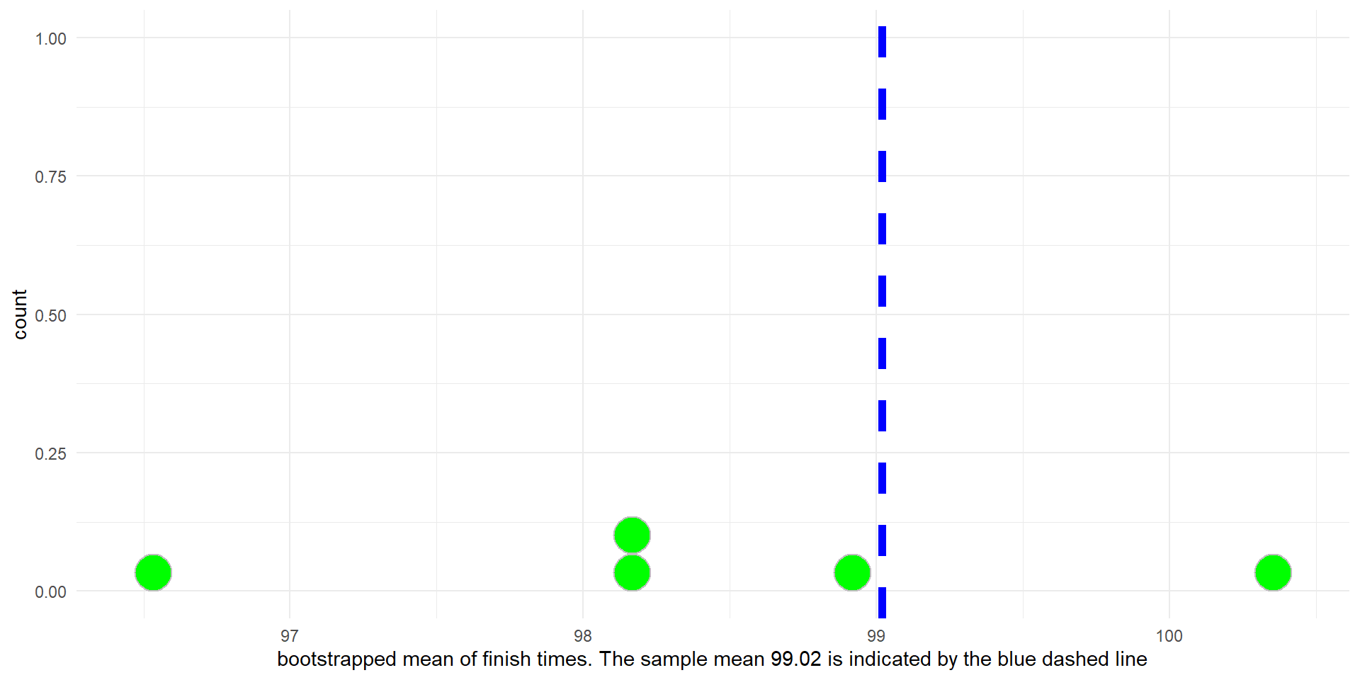
Histrogram showing 5 bootstrapped means.

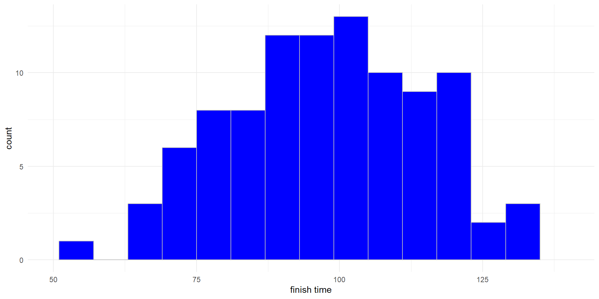
Here is the result of 1,000 bootstapped means.

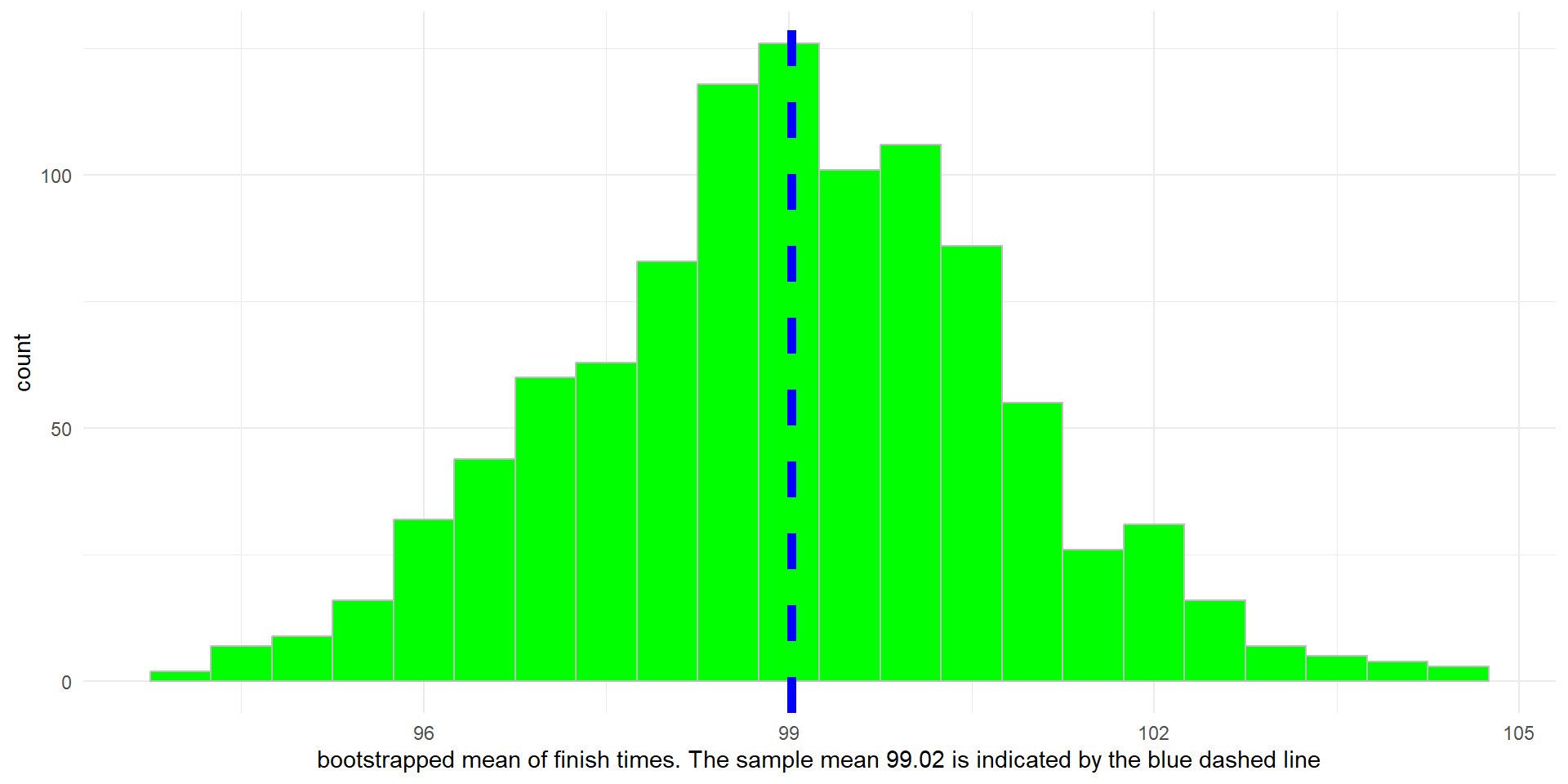
Histrogram showing 1,000 bootstrapped means.

Variability in the data vs variability of the mean

Distribution of 10-mile finish times(the actual data of the sample of 100 runners).
run17 |>
  summarize(sd_data = sd(time))

Result of 1,000 bootstrapped means on the same horizontal axis.
run_boot |>
  summarize(se_means = sd(stat))
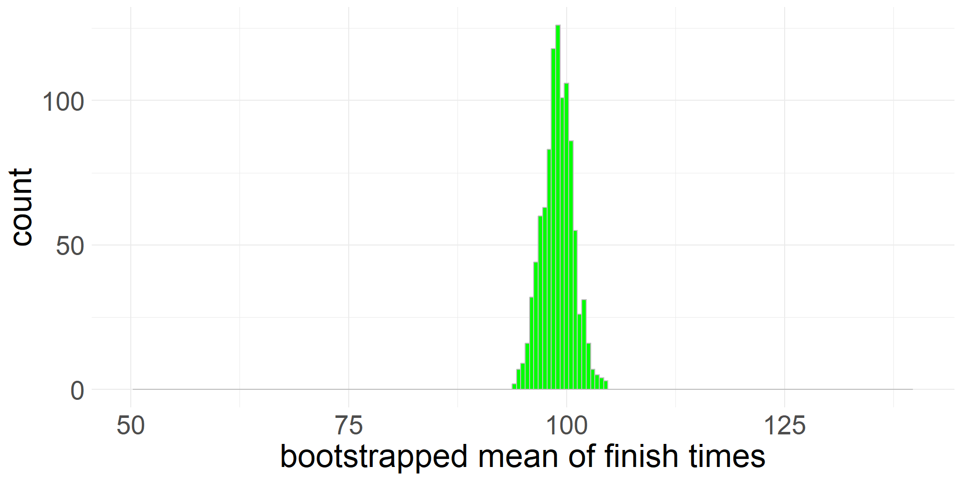
  • The standard deviation of the means (1.78) is the value of the standard error(SE)
  • Note that \(1.78\approx \frac{17.9}{\sqrt{100}}\)

Bootstrap SE Confidence Interval for the Mean

  • If bootstrap distribution is approximately symmetric and bell-shaped, we can calculate a confidence interval using the bootstrap SE. The value of the test statistic (sample mean \(\bar{x}=99.02\)) is the center of the CI.
  • A 95% bootstrap SE confidence interval for the mean finish time is \[ \begin{array}{rcl}\bar{x} \pm 1.96\times SE &=& 99.02 \pm 1.96\times1.78\\ &=& 99.02\pm3.49\end{array}\]
  • Thus, we are 95% confident that the mean finish time in 2017 is between 95.53 and 102.51 minutes
  • Note that we used the multiplier \(1.96\) that is based on the normal approximation, however the mathematical model of this analysis will be based on a different distribution (called t-distribution)

Bootstrap Percentile CI for the Mean

  • We can also calculate a bootstrap percentile confidence interval for the mean

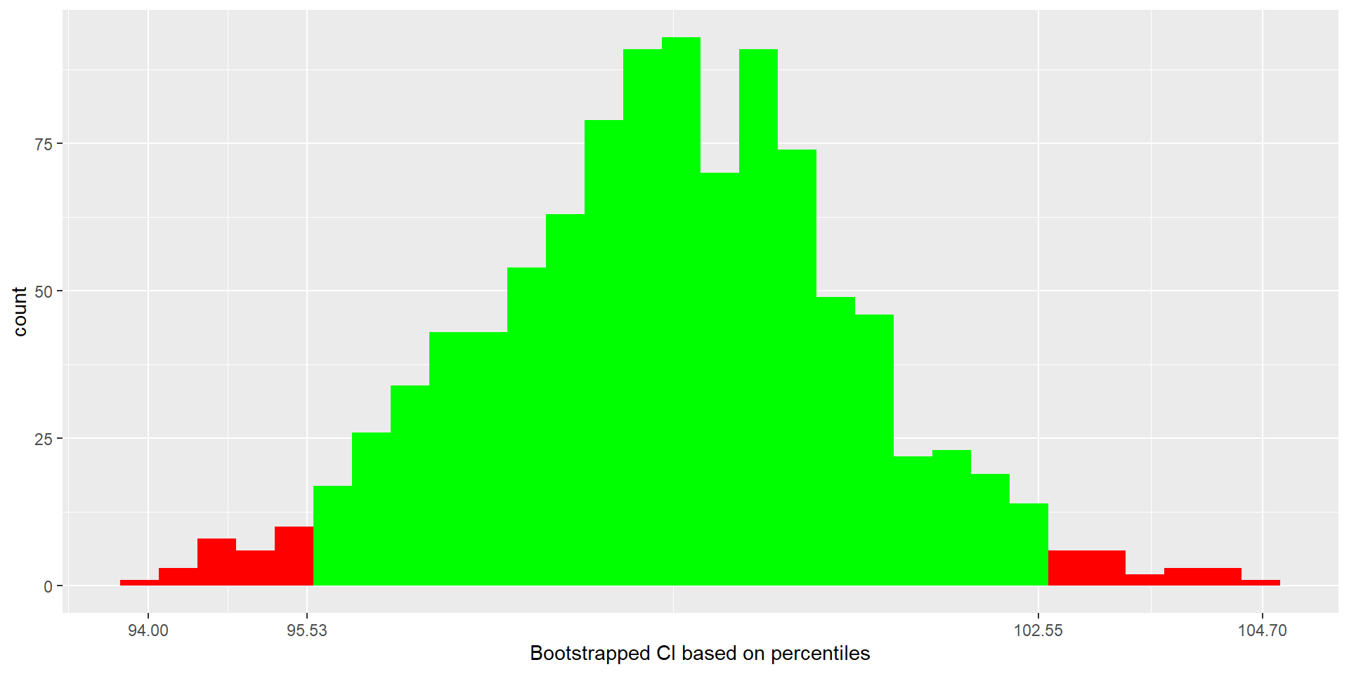
  • A 95% bootstrap percentile confidence interval for the mean finish time is (95.53, 102.55)

Mathematical Model for Distribution of Means

Central Limit Theorem for Sample Mean

When the following conditions are met, the sampling distribution of \(\bar{x}\) from for samples of size \(n\) from a population with mean \(\mu\) and standard deviation \(\sigma\) will be approximately normal with mean = \(\mu\) and standard error \[SE=\frac{\sigma}{\sqrt{n}}\]

  1. Independent observations
  2. Normality: when sample is small, sample observations must come from a normally distributed population. When sample is large, this condition can be relaxed.

We can use this rule of thumb for the normality check:

  • If \(n<30\) and there are no clear outliers, then we usually assume the data come from a nearly normal distribution to satisfy the condition.
  • If \(n\geq30\) and there are no particularly extreme outliers, then we usually assume the sampling distribution of \(\bar{x}\) is nearly normal, even if the underlying population distribution is not
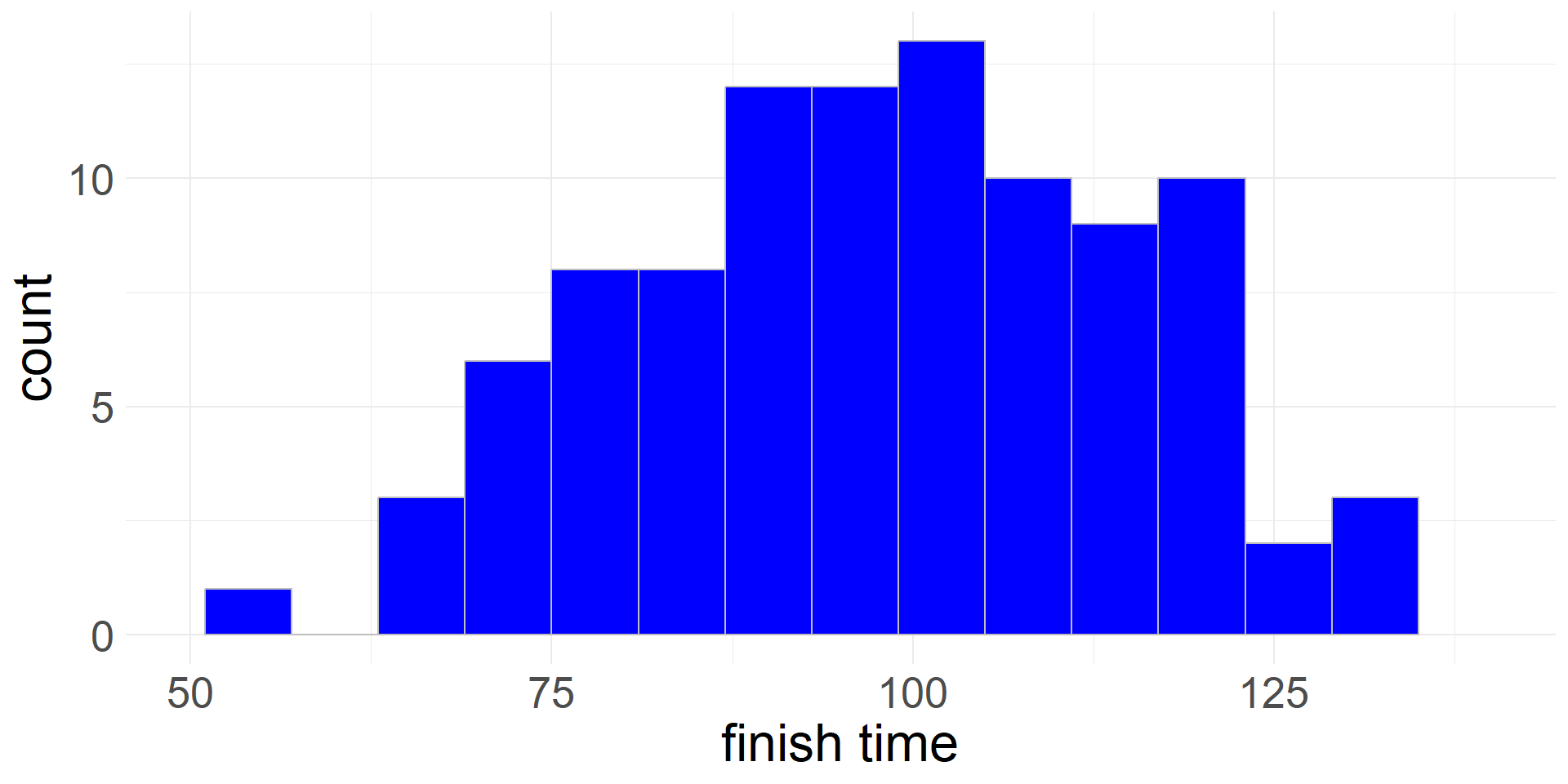
  • The Cherry Blossom run data satisfy the normality check, since there are 100 (so \(n\geq 30\)) observations, and no particularly extreme outliers
  • The observations are independent, because they come from a simple random sample (SRS) of finishers

T-distribution

  • In order to estimate the SE using the formula, we need to estimate the population standard deviation \(\sigma\)
  • The best estimate is the sample standard deviation \(s\) \[SE = \frac{\sigma}{\sqrt{n}}\approx\frac{s}{\sqrt{n}}\]
  • The test statistic for assessing a single mean is \(T\) \[T=\frac{\bar{x}-null\,value}{s/\sqrt{n}}\]

T-Distribution

Mathematical Model for \(T\)

The \(T\) statistic (\(T\) score) will have will have a \(t\)-distribution with \(df=n-1\) degrees of freedom if the following conditions are met:

  1. Independent observations
  2. Large samples with no extreme outliers (use same rule of thumb)
  • The tails of the \(t\)-distribution are thicker than the normal distribution due to uncertainty in the SE estimate
  • This is especially true for smaller samples

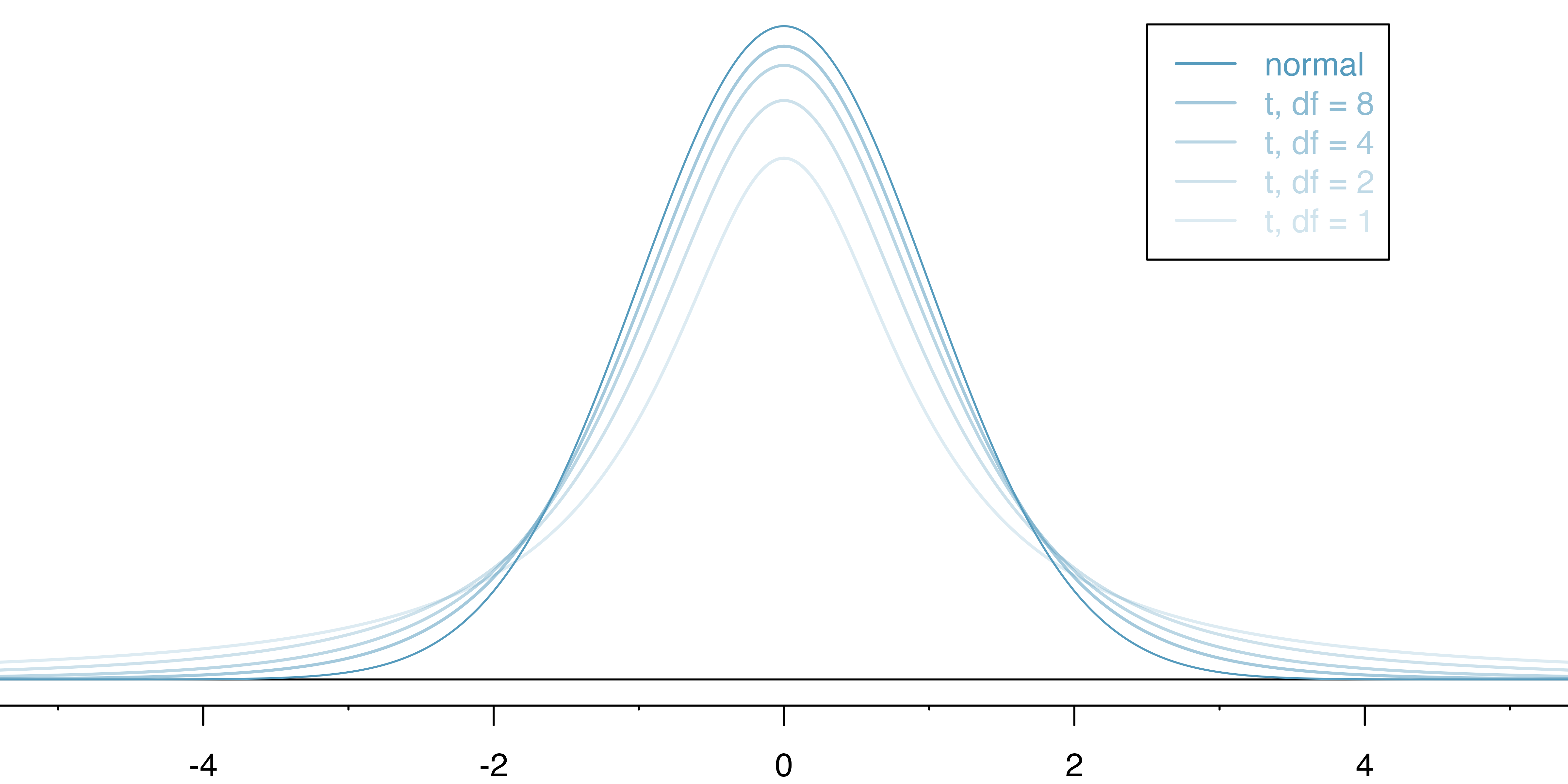
Comparison of normal distribution and \(t\)-distributions with different degrees of freedom (IMS2 Figure 19.9).

One Sample T-Interval

  • If the conditions are met, we can use the \(t\)-distribution to calculate a confidence interval, called a one sample t-interval
  • The interval is \[\bar{x}\pm t^{\ast}_{df}\times \frac{s}{\sqrt{n}}\]
  • The value of \(t^{\ast}_{df}\) depends on the confidence level and degrees of freedom
  • For the Cherry Blossom run finish times, \(df=100-1=99\)
  • To find \(t^{\ast}_{99}\) for a 95% confidence interval we find the cutoff for the \(t\) distribution that gives us 95% in the middle
  • In Jamovi: Randomize - > Model-Based Inference
  • We find that \(t^{\ast}_{99}=1.98\)

  • Thus the 95% confidence interval is \[99.02\pm 1.98\times \frac{17.93}{\sqrt{100}}\]

  • The bounds of the 95% one sample t-interval are (95.46, 102.56)

Comparison of Confidence Intervals

Type 95% CI
One sample \(t\)-interval (95.46, 102.56)
Bootstrap SE (95.51, 102.49)
Bootstrap percentile (95.53, 102.55)

One Sample T-Test

  • If the conditions are met, we can use the \(t\)-distribution to conduct a hypothesis test
  • Recall that we want to determine of the average finish time is different than it was in 2006 (93.29 min)
    • \(H_0: \mu = 93.29\)
    • \(H_A: \mu \neq 93.29\)
  • The \(T\)-statistic is \[\begin{array}{lcr}T &=& \frac{\bar{x}-null\,value}{s/\sqrt{n}} &=& \frac{99.02-93.29}{17.93/\sqrt{100}} &=& \frac{99.02-93.29}{1.793} &=& 3.20 \end{array}\]

  • Since the alternative hypothesis is two-sided, the p-value is the total area under two symmetric tails of the density curve for \(t_{99}(\)the \(t\)-distribution with \(df=99\)) as extreme as the test statistic \(T\)

    • (\(\leq-3.2\) or \(\geq3.2\))
  • We find the area in the left tail using pt and double it (the t-distribution is symmetric)

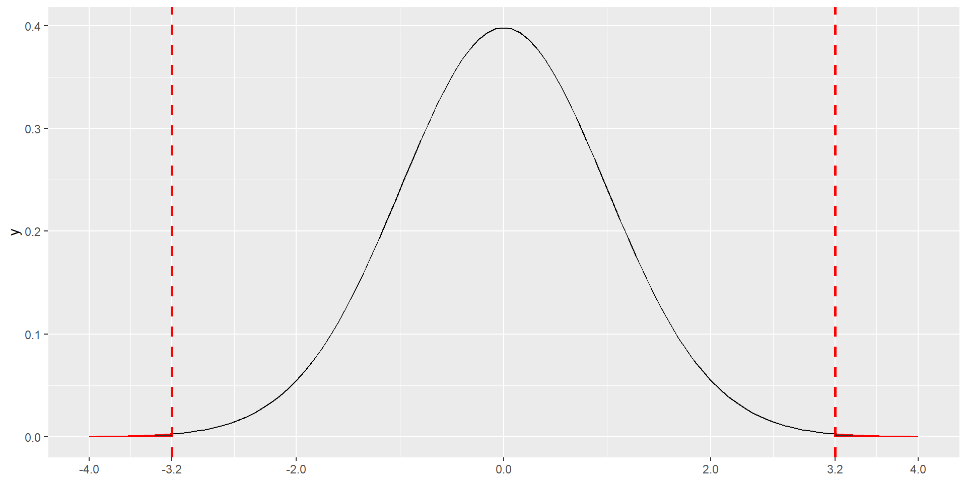
t-distribution with 99 d.f.

  • In Jamovi: Randomize - > Model-Based Inference

Conclusion

  • We are able to reject the null hypothesis at the \(\alpha = 0.05\) significance level.
  • We conclude that the mean finishing time in 2017 is different than 93.29 minutes (in fact, it is higher, so the runners are getting slower)
  • We can generalize this result to a larger population since it was a random sample
  • Note that this result is consistent with the 95% confidence intervals (say, t-interval was (95.46, 102.56))
  • 93.29 minutes is not considered a plausible value for the mean based on the CI
  • We almost always get consistent results between a two-sided hypothesis test with significance level \(\alpha\) and a confidence interval with confidence level \((1-\alpha)\times 100 \%\)
    • if we reject the null hypothesis with \(\alpha=0.05\), the null value will not be included as a plausible value in the 95% CI

    • if we fail to reject the null hypothesis with \(\alpha=0.05\), the null value will be included as a plausible value in the 95% CI

Blood Pressure

  • A sample of 50 adult participants completed an 8-week lifestyle intervention designed to improve cardiovascular health.

  • The variable of interest is systolic blood pressure (mmHg) measured at the end of the program.

  • The dataset contains a single quantitative variable (Systolic_BP), representing each participant’s post-intervention reading.

  • The data set systolic_bp available here

  • Researchers aimed to test whether the average systolic blood pressure after the program differs significantly from the clinical benchmark of 120 mmHg.

    • Run single mean test of significance
    • Make full conclusion
    • Find 95% confidence interval and interpret it
    • Is the CI consistent with the test of significance?