 χ² Tests
 ─────────────────────────────────────
         Value       df    p
 ─────────────────────────────────────
   χ²    18.96998     4    0.0007967
   N          149
───────────────────────────────────── Inference: Two-Way Tables
Chapter 18
Math 115
Math 115
Let us begin plotting the resulting \(\chi^2\) values on the dotplot:
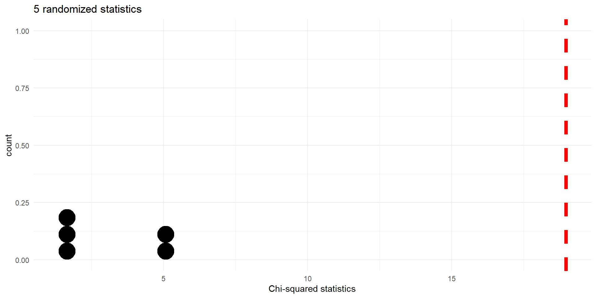
Histogram of \(X^2\) statistics for 5 random permutations. Observed value (\(18.97\)) indicated by dashed vertical line.
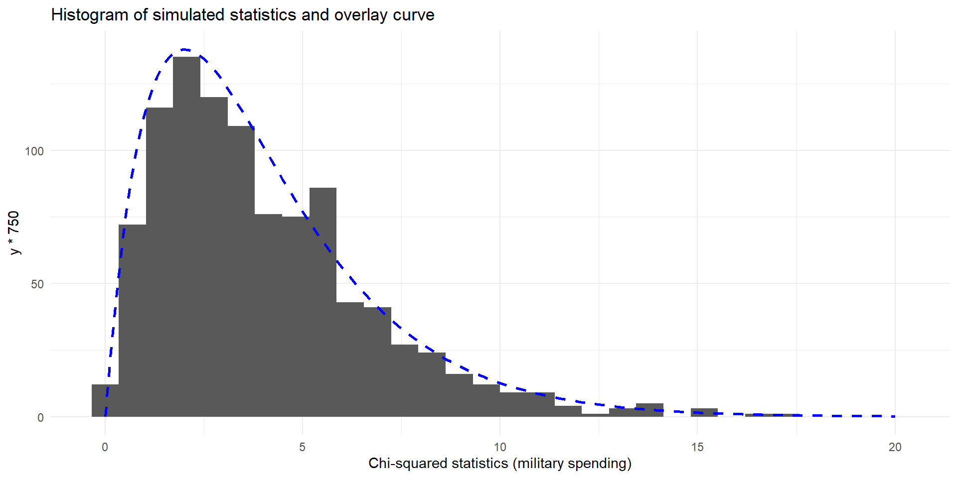
Here is the resulting histogram of 1,000 simulations
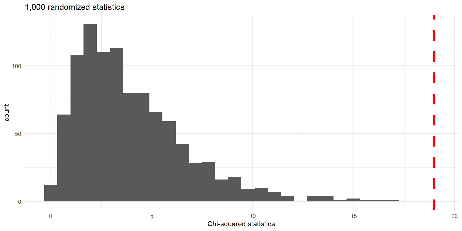
Histogram of \(X^2\) statistics for 1,000 random permutations. Observed value (\(18.97\)) indicated by dashed vertical line.
- Note that the shape of the histogram is neither symmetric nor bell-shaped. In fact, it only uses non-negative values
- Both two-way tables satisfy the large samples condition (at least 5 expected counts in each cell)
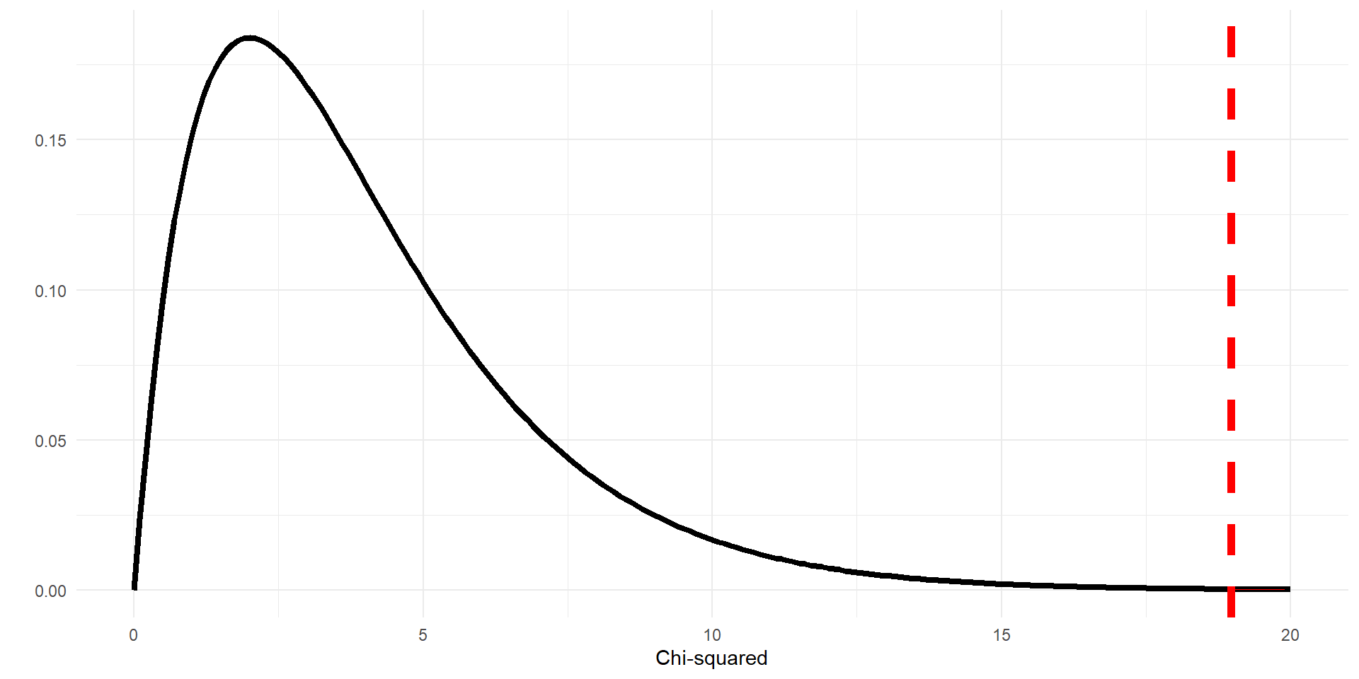
- In both cases there are 3 rows and 3 columns in the table, so \(df=(r-1)\times(c-1)=(3-1)\times(3-1)=4\)
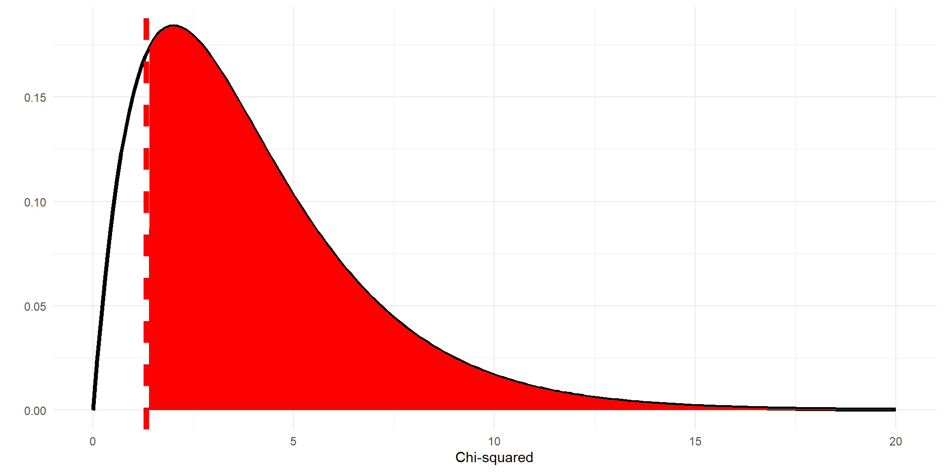
- The p-value is the area under the curve that is beyond the observed \(X^2\) value
- Here the the p-value for the hypothesis test on military spending
- Here is Jamovi output
 χ² Tests
 ─────────────────────────────────────
         Value       df    p
 ─────────────────────────────────────
   χ²    18.96998     4    0.0007967
   N          149
 ─────────────────────────────────────
Test of Significance
| Party | TOO LITTLE | ABOUT RIGHT | TOO MUCH | Total |
|---|---|---|---|---|
| Dem | 8 | 22 | 13 | 43 |
| Ind | 13 | 37 | 22 | 72 |
| Rep | 9 | 17 | 8 | 34 |
| Total | 30 | 76 | 43 | 149 |
| Party | TOO LITTLE | ABOUT RIGHT | TOO MUCH | Total |
|---|---|---|---|---|
| Dem | 8 (8.66) | 22 (21.93) | 13 (12.41) | 43 |
| Ind | 13 (14.50) | 37 (36.72) | 22 (20.78) | 72 |
| Rep | 9 (6.85) | 17 (17.34) | 8 (9.81) | 34 |
| Total | 30 | 76 | 43 | 149 |
Use Jamovi to calculate \(\chi^2\) statistic
 χ² Tests
 ─────────────────────────────────────
         Value       df    p
 ─────────────────────────────────────
   χ²    1.326060     4    0.8569388
   N          149
───────────────────────────────────── 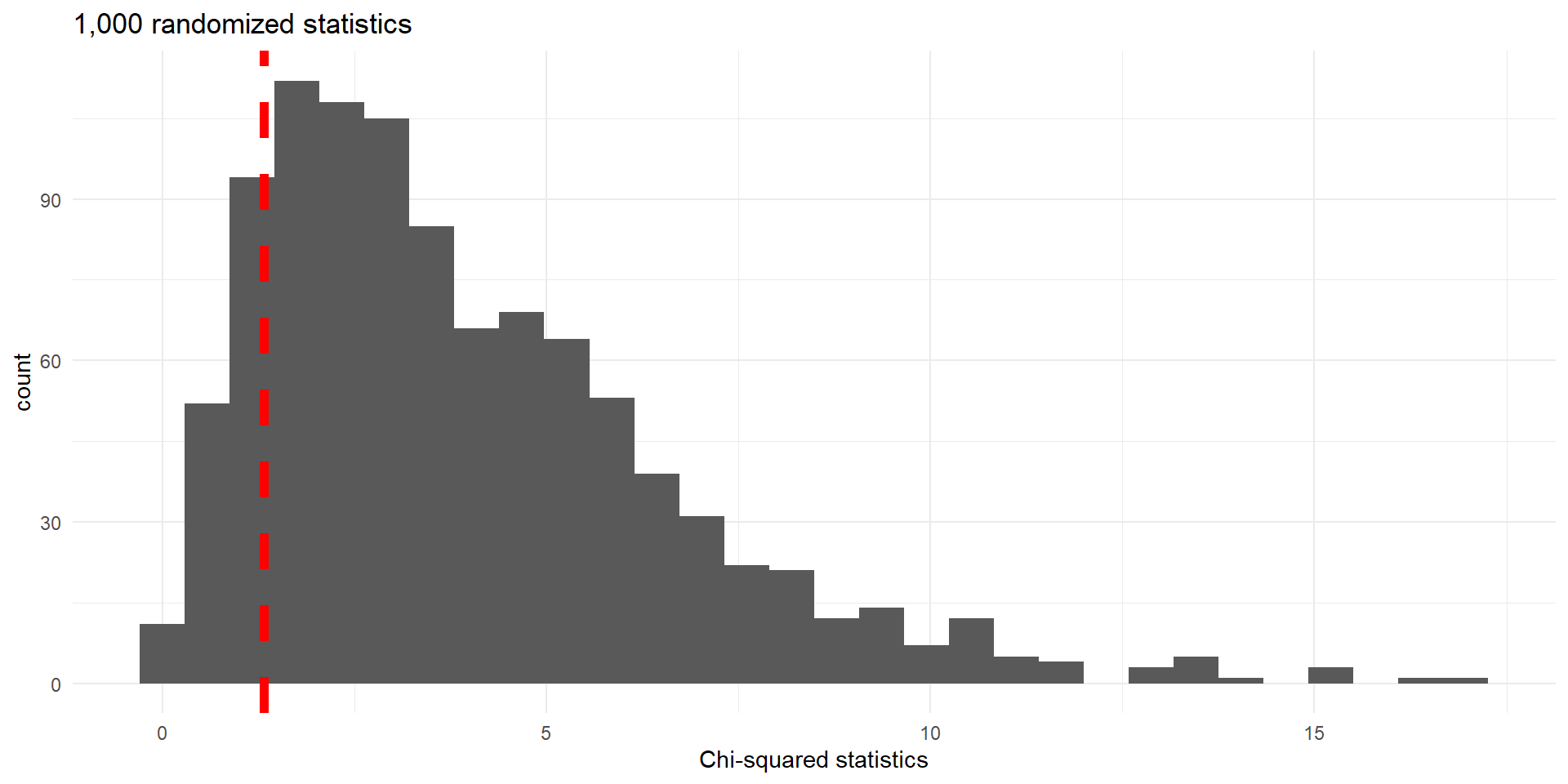
\(X^2\) statistics for 1,000 random permutations. Observed value (\(1.326\)) indicated by dashed vertical line.
 χ² Tests
 ─────────────────────────────────────
         Value       df    p
 ─────────────────────────────────────
   χ²    1.326060     4    0.8569388
   N          149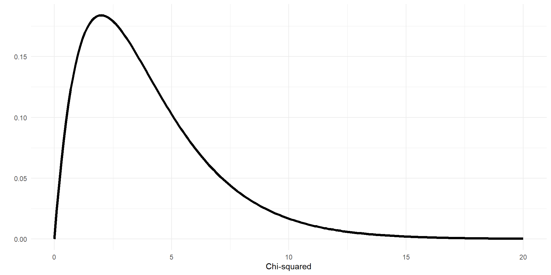
───────────────────────────────────── \(X^2\) distributions for different \(df\)
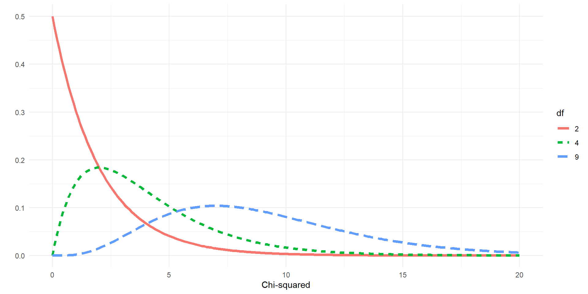
Chi-squared disributions with different degrees of freedom (df).
- Chi-squared distribution is more peaked for lower \(df\)
- Thicker tail for higher \(df\)
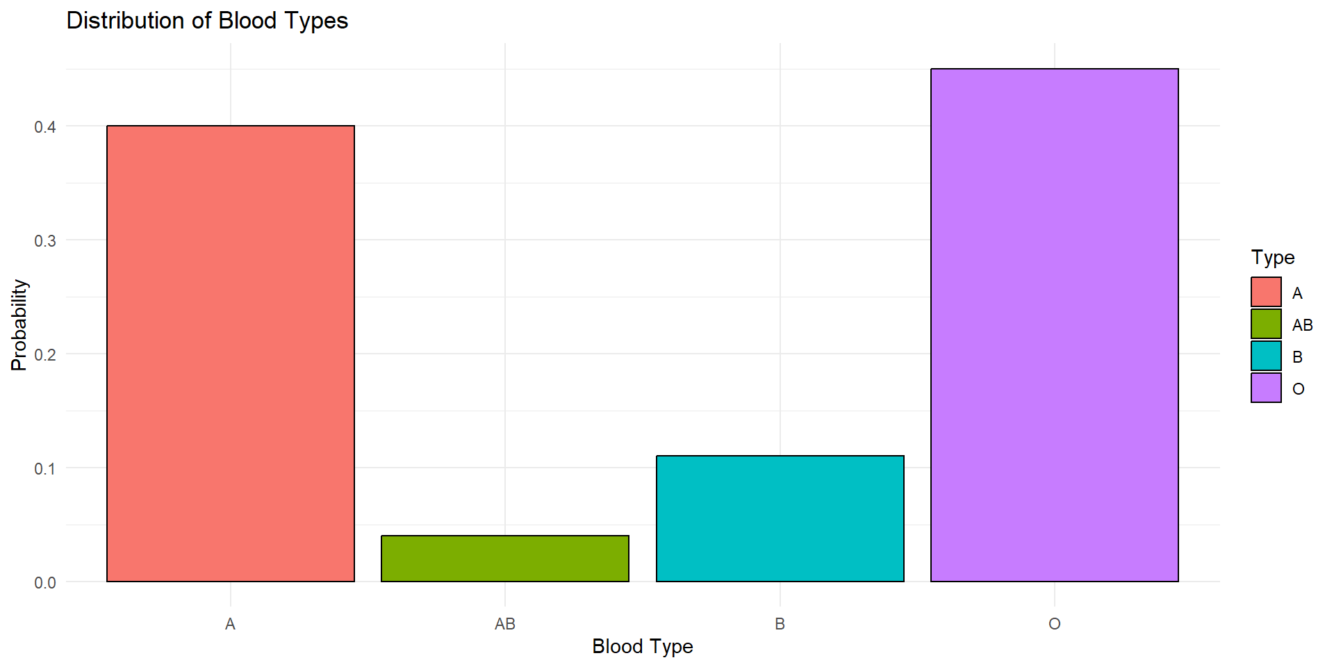
Blood Type Example
- Assume that the expected probabilities of various blood types in the general population are:
A = 0.40, B = 0.11, AB = 0.04, O = 0.45
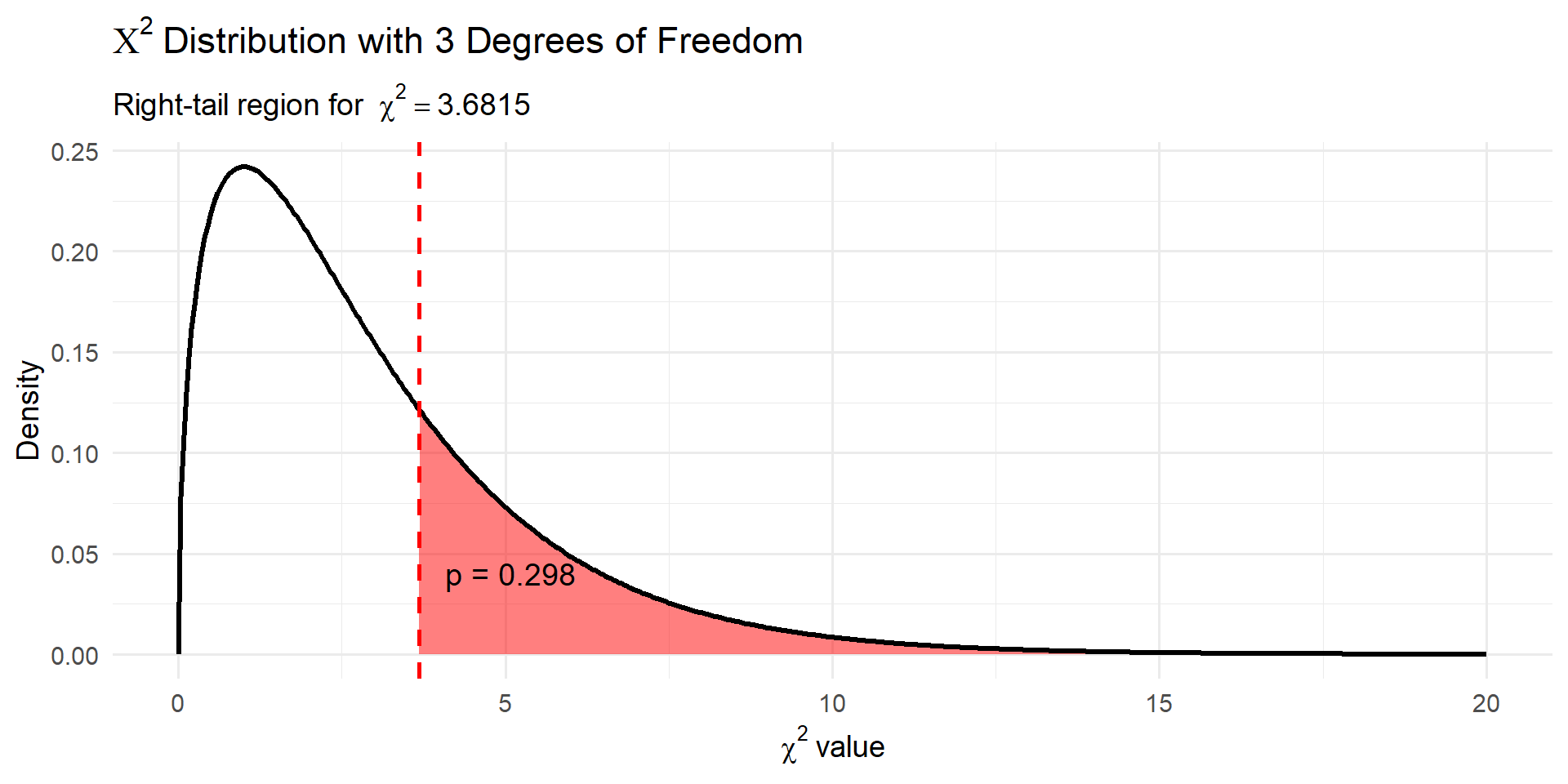
Chi-Square distribution and p-value
| Chi_Square | DF | P_Value |
|---|---|---|
| 3.6815 | 3 | 0.298 |