Inference for a Single Proportion

Chapter 16
Math 115

Two data sets

We will consider two data sets:
- First is on payday loan regulations in MI (payday)
- Second is on the complication rate for liver donor surgeries in the U.S. (consult)
We will use the first data set as an example of an inference based on a mathematical model and second as an example of a simulation based inference
The decision in each case is based on the success-failure condition (also known as the validity condition) of the Central Limit Theorem

Mathematical Model for a Proportion

We have learned that if certain conditions are met we can use a mathematical model to make inferences about a population
There is a version of the Central Limit Theorem for a single proportion

Sampling distribution of \(\hat{p}\)

The sampling distribution of \(\hat{p}\) based on a sample of size \(n\) from a poplation with true proportion \(p\) will be approximately normal with mean \(p\) and standard error \[SE=\sqrt{\frac{p(1-p)}{n}}\]
if the following technical conditions are met:

independent observations (e.g., observations from SRS)
(success-failure condition) at least 10 expected successes and at least 10 expected failures. (i.e., \(np\geq 10\) and \(n(1-p)\geq 10\))

Payday Loan Regulations

Borrowers use payday loans to get a cash advance before their next payday
Borrower writes a check for loan amount + service fee
Lender holds check until borrower’s payday
Very high APR equivalent (often over 300%)
Some borrowers take out second loan to pay of first, and so on

Michigan already has a law that limits the number of payday loans a borrower can hold (2)
Do most payday borrowers support additional regulation that would require payday lenders to do a credit check?
Let \(p\) be the long-run proportion of all payday borrowers in MI that support additional regulation.
Note that \(p\) represents a population parameter

Hypotheses

In words:

\(H_0:\) the proportion of all payday borrowers in MI that support additional regulation is 50%.
\(H_A:\) The majority of all payday borrowers (more than 50%) in MI that support additional regulation.

In symbols:

\(H_0: p = 0.5\)
\(H_A: p > 0.5\)

Data

payday data set is available here
Researchers selected a random sample of 826 payday borrowers
- 424 (51.3%) said they would support a regulation
- \(\hat{p}=0.513\)
- Null hypothesis assumes true value of the population proportion \(H_0: p= 0.5\)
The success-failure condition is met:
- Under the null hypothesis, we expect \(n\times p=0.5\times 826 = 413\) people to support the legislation
- \(n\times (1-p)=(1-0.5)\times 826 = 413\) to not support the legislation.
It is appropriate to model the null distribution of \(\hat{p}\) using a normal distribution

Hypothesis Test Using Normal Approximation

The standard error, according to the CLT is \[SE(\hat{p})=\sqrt{p_0(1-p_0)/n}\] Where \(p_0\) is the proportion under the null hypothesis (so, in our example \(p_0=0.5\))
We will use the Z score as the test statistic

\[Z = \frac{\hat{p}-p_0}{SE(\hat{p})}=\frac{\hat{p}-p_0}{\sqrt{p_0(1-p_0)/n}}\]

Recall that if \(\hat{p}\) is normally distributed, then \(Z\) has a standard normal distribution, \(N(0,1)\)

For the payday study \(p_0=0.5\), and \(\hat{p}=0.513\), so \[SE(\hat{p})=\sqrt{\frac{p_0(1-p_0)}{n}}=\sqrt{\frac{0.5\cdot(1-0.5)}{826}}=0.0174\]
So the Z-score is \[Z = \frac{0.513 - 0.5}{0.0174}=0.765\]

The p-value is the probability that we would obtain a \(Z\) score at least as large as 0.765 if the null hypothesis is true
We compute the p-value by finding the area under the density curve for \(N(0,1)\) that is beyond 0.765

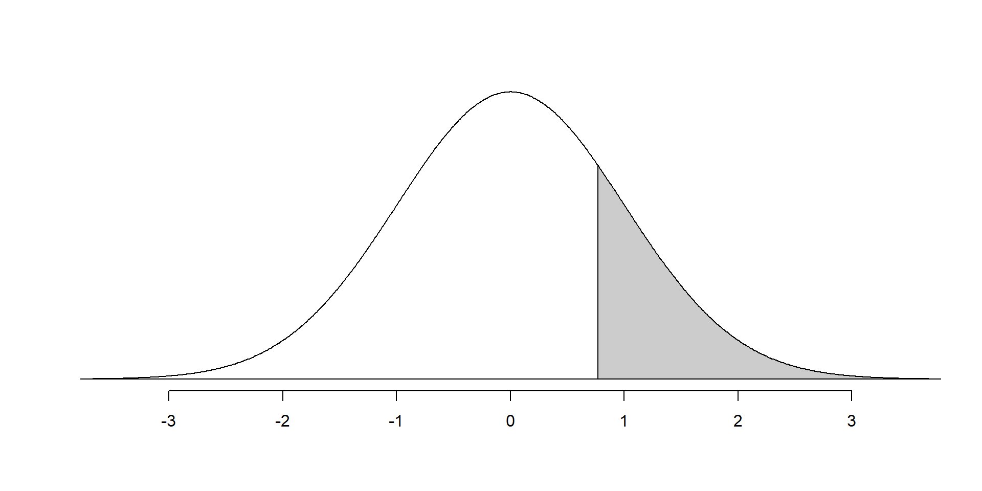
Standard Normal model, \(N(0,1)\). P-value is area of shaded region.

The p-value of the test is 0.22214

So the evidence was not strong enough to reject the null hypothesis (p-value = 0.22)
Therefore, 50% is a plausible value for the parameter
Note that we cannot claim that 50% of payday borrowers support the new legislation (we cannot accept the null hypothesis)
We state that we failed to reject null hypothesis.

Confidence Interval

We can also use a normal distribution to find a confidence interval if technical conditions are met
Earlier we used \(p_0\) as the mean and in the computation of SE, because we were trying to approximate the null distribution
A confidence interval estimates the value of the parameter, so it only can rely on the sample data
The best point-estimate we have is the sample proportion \(\hat{p}\), so we use that in the computation of SE

Checking Conditions for CI

The success-failure condition is easier to check in this situation.
\(n\hat{p}\) is the number of observed success, and \(n(1-\hat{p})\) is the number of observed failures.
We just need to check if there were 10 successes and 10 failures in the sample.
For the Payday loans study, the success-failure condition is met. There were 424 successes and 402 failures in the sample
It is appropriate to use a normal approximation to find a CI

Confidence Interval Using a Normal Approximation

If a normal approximation is appropriate, a confidence interval for a proportion can be written as \[\hat{p}\pm z^{\ast}\times SE\]
SE is estimated using \[SE\approx\sqrt{\frac{\hat{p}(1-\hat{p})}{n}}\]
\(z^{\ast}\) is determined by the confidence level (e.g., 1.645 for 90%, 1.96 for 95%, 2.576 for 99%)

The standard error for the proportion of borrowers that support the new regulation is \[SE \approx \sqrt{\frac{0.513\cdot(1-0.513)}{826}}=0.0174\]
The 95% confidence interval is \[0.513\pm1.96\cdot0.0174 = 0.513\pm0.034\]
We are 95% confident that the long-run (or true) proportion of all payday borrowers that support the new regulation is between \(0.479\) and \(0.547\)
Note that value \(0.5\) used previously in the null hypohesis is inside of the 95% confidence interval, conforming the fact that 50% is a plausible value for the parameter

Preliminary example

Suppose that I want to see if a two-sided coin is fair
I flipped it 30 times and ended up with 21 heads and 9 tails
Is that strong evidence that the coin is not fair?
Simulations:
- I can simulate the flips of a fair coin
- I can repeatedly flip coins (30 times per simulation) and see what proportion will be heads
- After many such sequences of 30 I will see what is the sampling distribution of the proportion of heads
- On Moodle go to General Information -> Single Proportion Simulator

Simulation Based Inference

Medical Consultants
- Some organ donors work with a medical consultant who helps them throughout the process
- The average complication rate for liver donor surgeries in the United States is about 15%
- One consultant claims she has low rate of complications compared to national average.
Is her claim supported?
- Let \(p\) be the consultant’s long-run complication rate

Hypotheses:

\(H_0: p = 0.15\)
\(H_A: p < 0.15\)

Data:

consult dataset is available here
She has served as a consultant for 62 liver donor surgeries
- 3 (4.8%) resulted in complications
- \(\hat{p} = 0.048\)

Checking Technical Conditions

Consultant study

The success-failure condition is not met. Under the null hypothesis, we expect \(62\times 0.15 = 9.3\) complications (less than 10), even though the number of failures (\(62\times0.85=52.7\)) is greater than 10.
Cannot model null distribution using a normal distribution
Use randomization instead (parametric bootstrap simulation)

Hypothesis Test Using Randomization

In the consultant study we cannot use a normal model for the null distribution
However, we can use parametric bootstrap simulation to approximate the null distribution
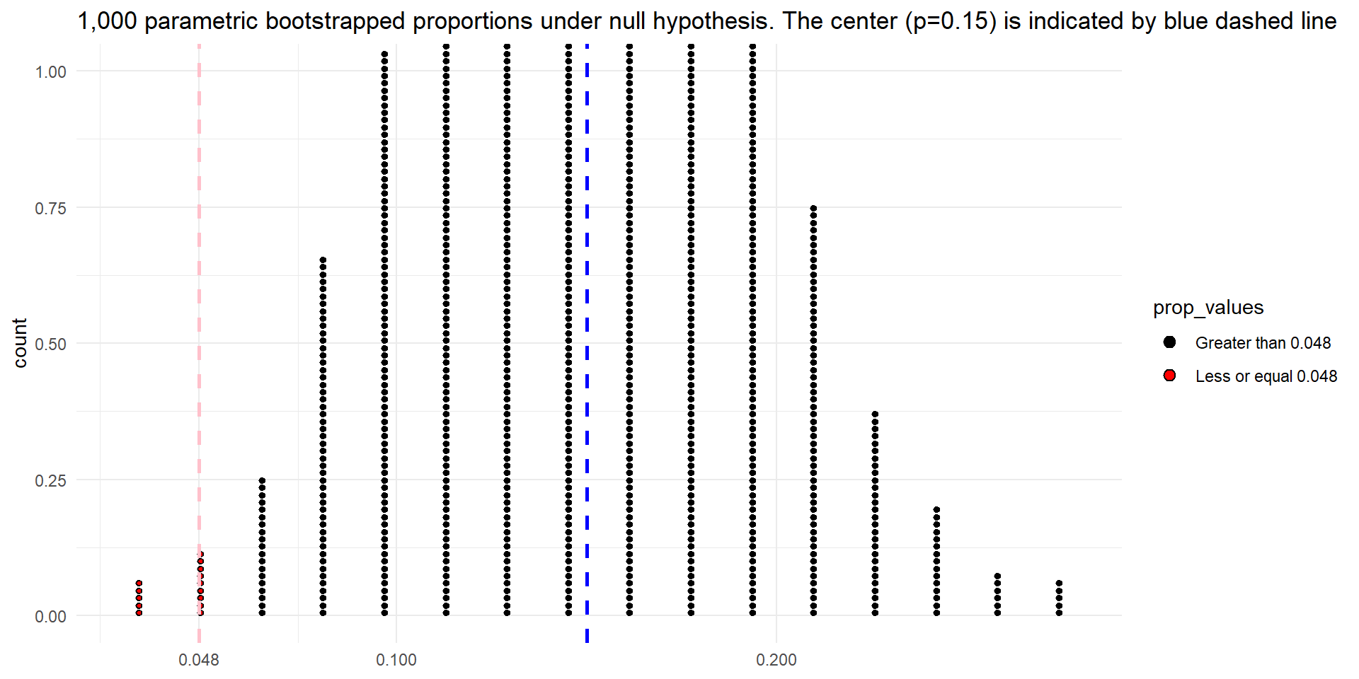
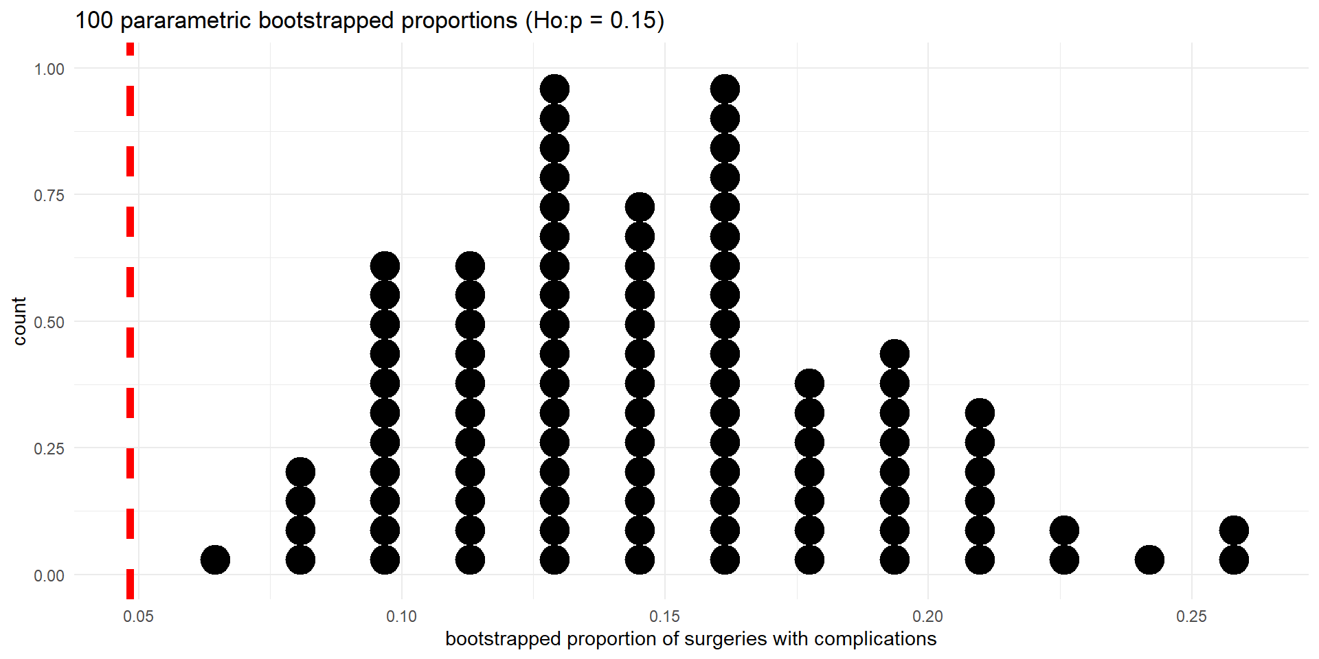
We simulate 1,000 random samples of 62 liver donors from a population in which the null hypothesis is true (10% complication rate)

Parametric bootstrap simulation is equivalent to the following physical simulation:

For each donor simulate the outcome by spinning a spinner with 15% of the area representing “complication” and 85% representing “no complication”
For each sample, spin the spinner 62 times (sample size) and record the proportion of complications in the sample
Repeat to obtain proportions for 1,000 simulated samples

Here are the first 100 simulations with the test statistic (\(\hat{p} = 0.048\)) indicated by a dashed line

Approximate null distribution of 1000 simulations. The sample statistic (0.048) indicated by red dashed line.

The p-value is approximated by the proportion of bootstrapped proportions that are at least as extreme as the observed proportion (\(\leq 0.048\))
Note that since the alternative is in the form “less than”, p-value region is in the left tail

There are 14 “dots” in the p-value region, so p-value is \(\frac{14}{1000}=0.014\)
With a p-value of 0.014 we reject the null hypothesis.
In the context of the problem: We have strong confidence that the consultant has complication rate lower than 15%

Checking Conditions for CI

For the Consultant study, the success-failure condition is not met. There were 3 successes and 59 failures
Cannot use normal approximation to find a CI
Use randomization instead (bootstrap as in Chapter 12)

Confidence Interval Using a Bootstrapping

We use bootstrapping to find a 95% confidence interval for the complication rate for the medical consultant
This time we take repeated samples (with replacement) from our original sample

Let’s take a look at a 100 bootstrapped resamplings first

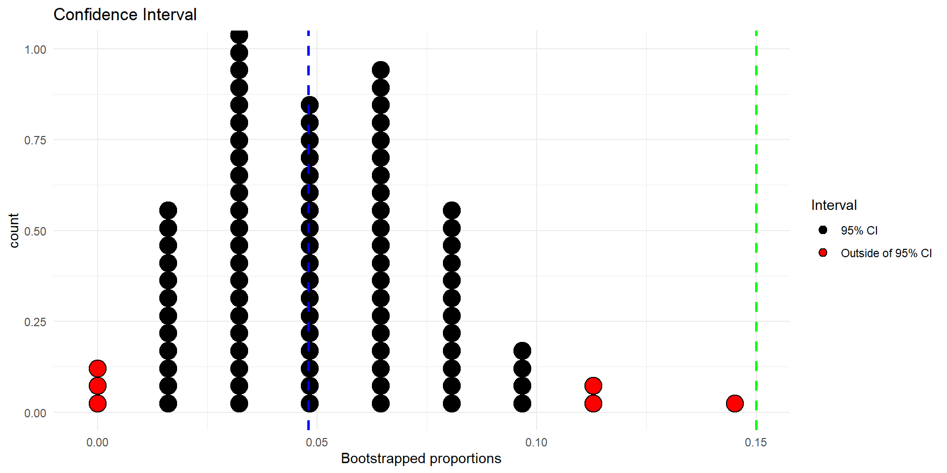
Test statistic \(\hat{p}=0.048\) (The center of the distribution)
Null hypothesis value (\(H_0:p=0.15\))

Histogram of the 1,000 bootstrap proportions using the sample (\(\hat{p}=0.048\))

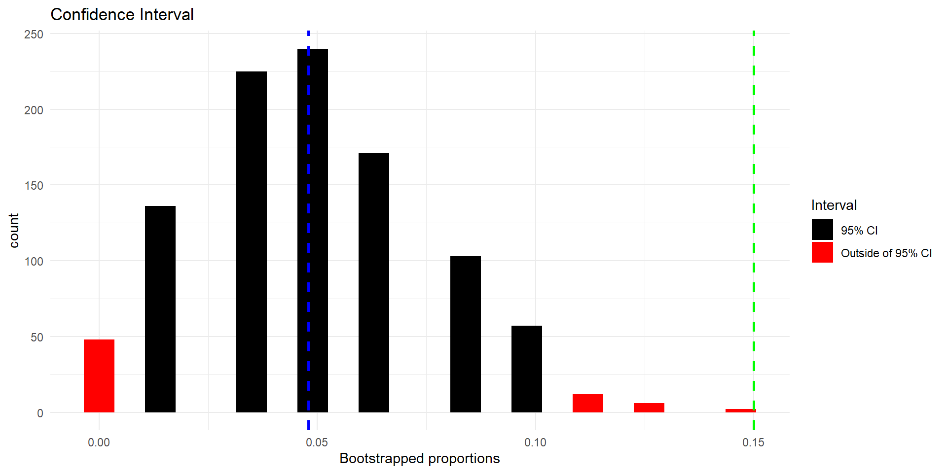
Test statistic \(\hat{p}=0.048\) (The center of the distribution)
Null hypothesis value (\(H_0:p=0.15\))

The 95 % bootstrap confidence interval is obtained by calculating the 2.5% and 97.5% percentiles for the bootstrapped statistics.
We are 95% confident that the consultant’s long-run complication rate is between 0 and 0.113
Note that the value we used in the null hypothesis (0.15) is not in the confidence interval, confirming that we rejected 15% as a plausible value for the parameter of interest using significance level \(\alpha=0.05\)