The difference of proportions (East Coast - West Coast) is positive
It may be an evidence that the East Coast population prefers cola more than population of the West Coast
It may also be that there is no real difference in preference in the populations, and the observed difference is just a random variation in the proportions in the sample of this size from the populations
A hypothesis test states these two possibilities formally as hypotheses then weighs them against each other using the results from the sample as evidence
Hypotheses
The null hypothesis, denoted \(H_0\), represents a skeptical perspective or a claim of no difference
The alternative hypothesis, denote \(H_A\), represents an alternative claim of difference.
As statisticians, we usually establish hypotheses before viewing the data in order to avoid bias
Depending on you research question, you can have \(H_A\) in form “\(<\)” or “\(\neq\)”
In this case we already stated the research question “Do people on the East Coast have a higher preference for cola than people on the West Coast?”
In words:
\(H_0:\) Location has no
effect on preference for
cola over orange soda.
\(H_A:\) There is a higher
preference for cola
on the East Coast than
on the West Coast.
In symbols:
\(H_0: p_E - p_W = 0\) \(H_A: p_E - p_W > 0\)
\(p_E\) and \(p_W\) are parameters (i.e. long-run proportions of all people who prefer Cola on the East Coast and the West Coast)
\(\hat{p}_E\) and \(\hat{p}_W\) are sample proportions
Null Distribution
We test the null hypothesis by comparing the observed value of the statistic to a null distribution
Null hypothesis states that there is no difference in the proportions of people who prefer cola in the populations of the East Coast and West Coast \(H_0: p_E - p_W = 0\)
At the same time, even if we assume that \(H_0\) is true, we wouldn’t expect that every sample from each population will have exactly the same proportion of cola drinkers for the West Coast and the East Coast
The difference of sample proportions, therefore, will vary from sample to sample
The null distribution is the distribution that describes those values
It is an example of a sampling distribution (distribution of a statistic, in our case, difference of sample proportions)
Null Distribution Using Random Permutation
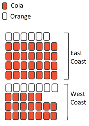
The sample data we collected represent the best available picture of the distribution of the drinkers on the coasts
Responses in the data
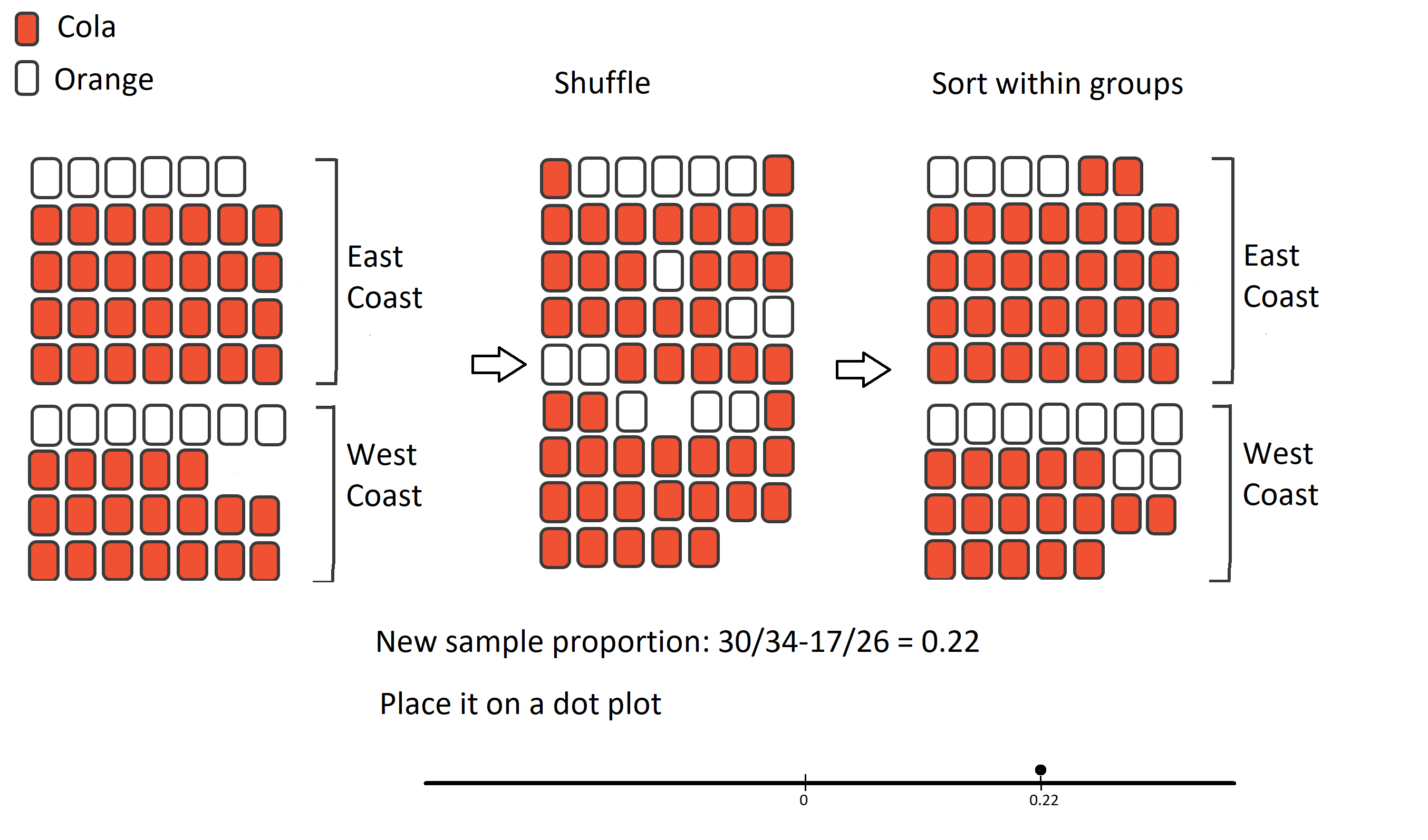
Random Permutation
To simulate the null hypothesis being true (no difference between West Coast and East Coast), I could shuffle the responses, split them into two piles according to sample sizes and calculate the new difference of sample proportions
If I do this many times it will give me a good idea of what the differences would look like if the null hypothesis is true (the null distribution)
Mixing up the values of the response variable is called random permutation
I can use random permutations to create a null distribution
Usually we will do this with a computer, because we want to calculate the statistic for 1,000 or 10,000 random permutations
Original Samples
Shuffling...
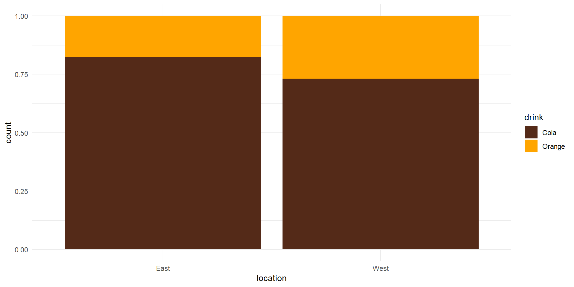
East Coast (34 people)
Cola: 28
Orange: 6
Proportion Cola: 0.824
West Coast (26 people)
Cola: 19
Orange: 7
Proportion Cola: 0.731
Difference in Proportions: 0.824 - 0.731 = 0.093← Original Data
Distribution of Differences
Red circle shows original difference (0.093). Blue circles show permutation differences.
Building the Null Distribution
Red line shows original difference (0.093). Gray bars show permutation differences.
Here is the original soda data with 5 random permutations.
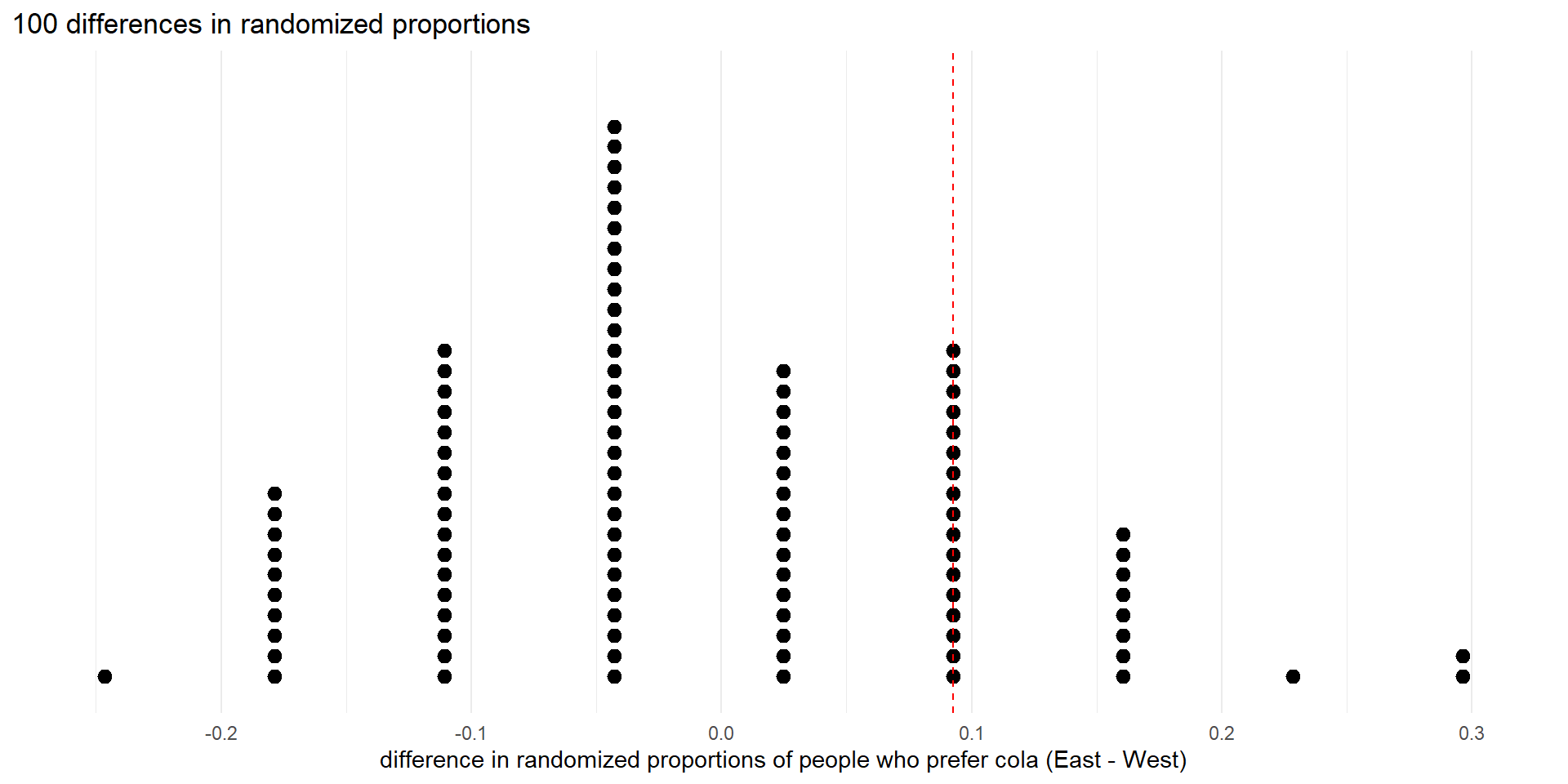
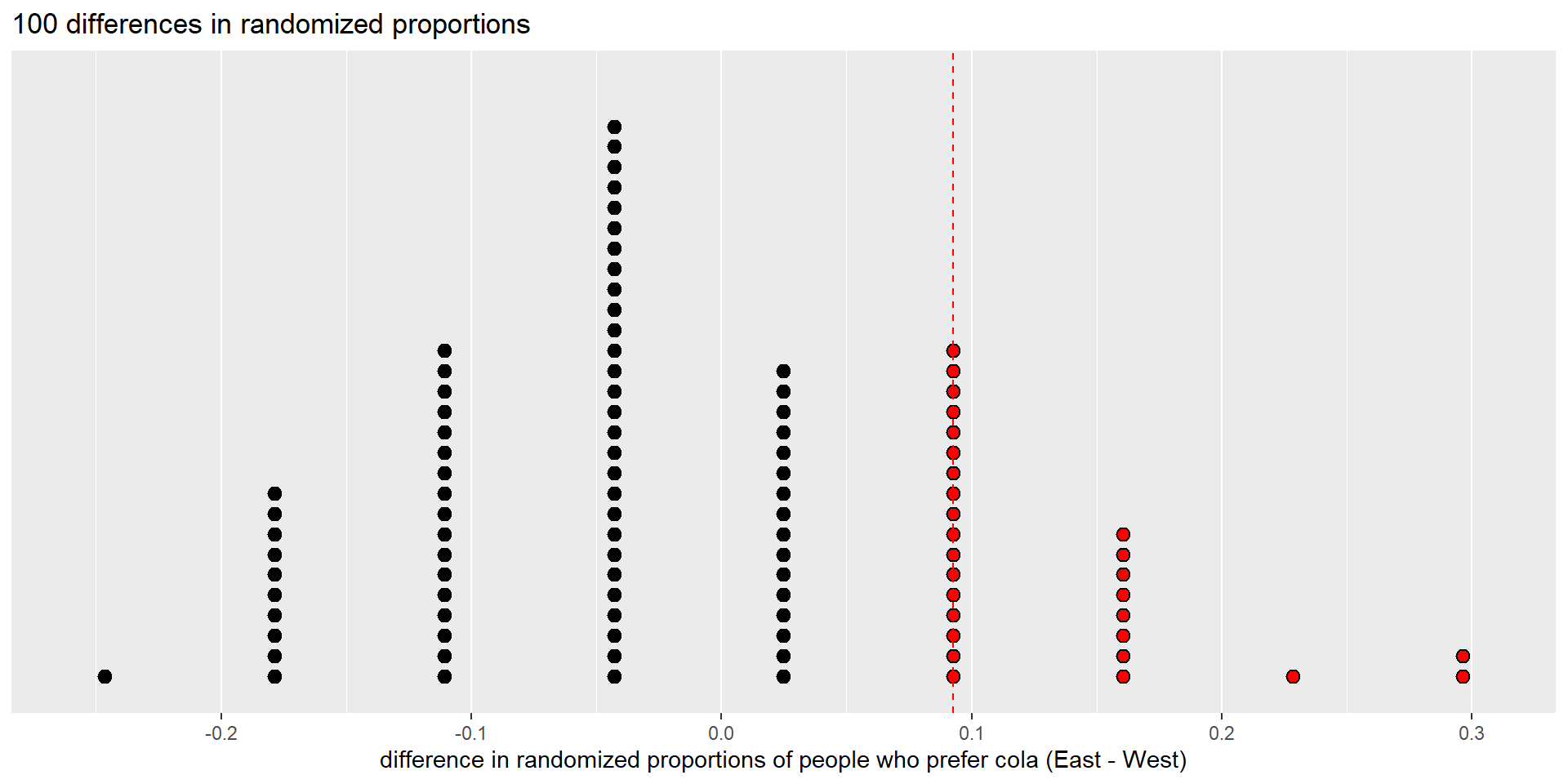
Now let’s simulate 100 samples assuming true null hypothesis
We’ll calculate a difference in proportions for each permutation
Later, we will learn how to do this in Jamovi
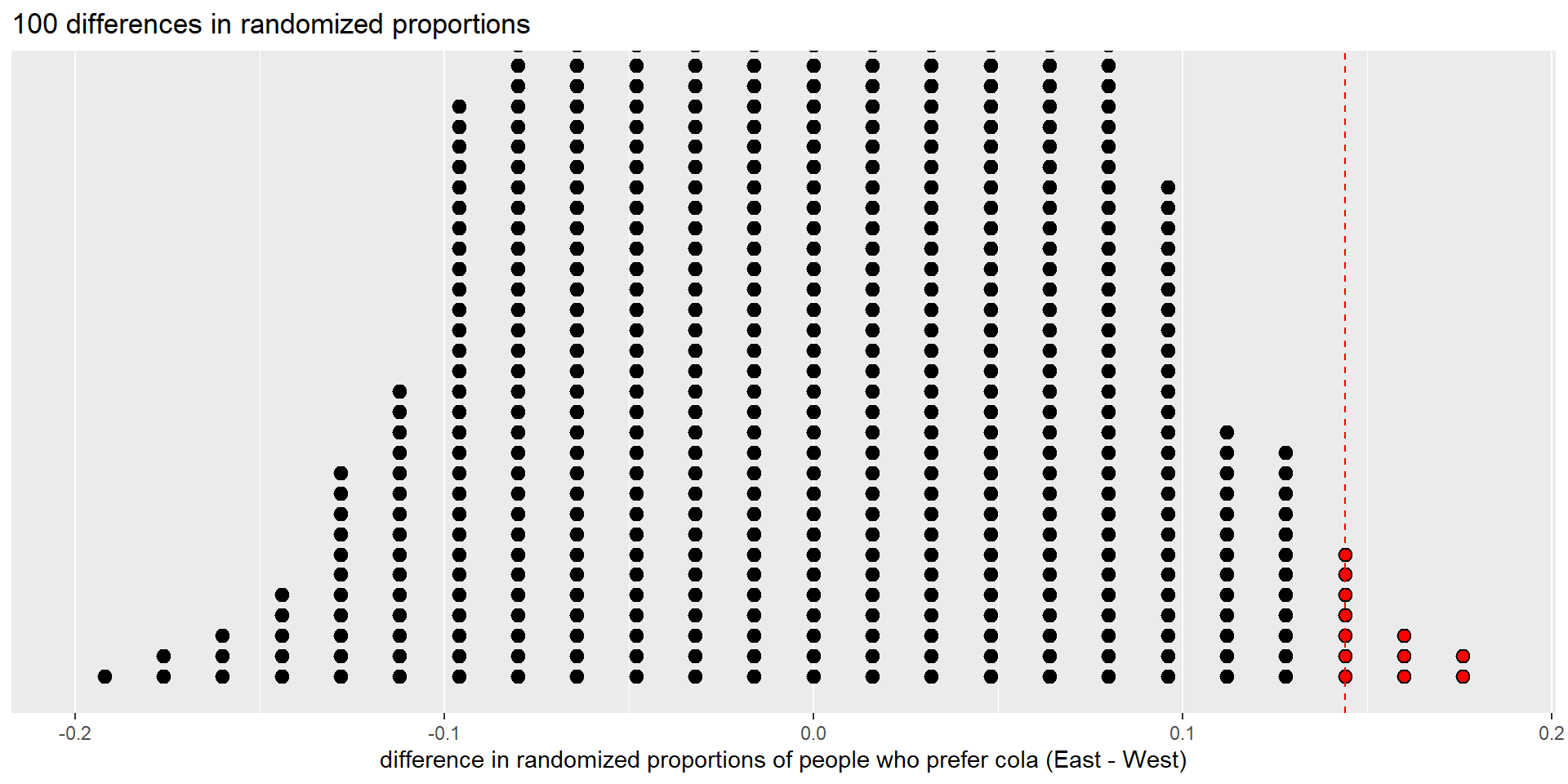
Dot plot of 100 differences in randomized proportions (null distribution), showing observed difference as dashed vertical line.
Red dots are as large or larger than the observed test statistic.
p-Value
To test the null hypothesis (\(H_0: p_E-p_W = 0\)) we consider how probable it would be to get a difference in proportions that is at least as large as the observed difference if \(H_0\) is true
This probability is called a p-value
We use the null distribution to calculate the p-value
The smaller is the p-value the stronger is the evidence against the null hypothesis.
There are 28 differences in randomization proportions that are greater than or equal to the observed value (0.09276). So we estimate the p-value to be 28/100 = 0.28.
The p-value is the proportion of red dots.
Significance Level
Before we conduct a study, we define a significance level, denoted \(\alpha\)
We decide that in order to reject the null hypothesis as false, the p-value must be less than \(\alpha\)
The significance level is the standard of evidence we will use to judge the null hypothesis
We presume the null hypothesis is true, but we are willing to reject it if the evidence against it is strong enough (the p-value is less than \(\alpha\))
Typical values for \(\alpha\) are 0.05 and 0.01
Sometimes other values are used
Unless otherwise noted, we will always use \(\alpha = 0.05\)
The significance level \(\alpha\) is the probability of rejecting the null hypothesiswhen it is true
The error that you make in this case is called Type I Error
Conclusion
In the soda example, the observed difference in proportions (\(\hat{p}_E-\hat{p}_W = 0.09276\)) does not allow us to reject the null hypothesis (p = 0.28) at the \(\alpha = .05\) significance level.
So, our formal conclusion is that we failed to reject the null hypothesis
The difference in the proportions is not statistically significant
This means that it is plausible that there is no difference in the proportions of people who prefer cola to orange soda between the East and West Coast.
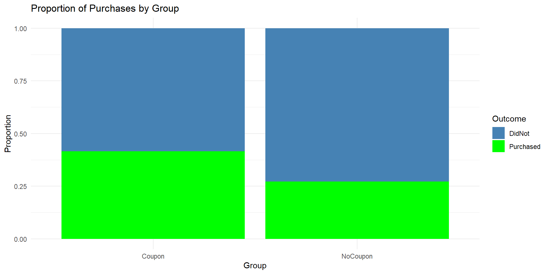
Consumer Behavior and Discount Offer
A marketing research firm conducted a randomized field survey to see whether a 10% discount coupon sent by email increases the probability that consumers will make a purchase in the following week. They randomly sampled 250 consumers and split them into two groups: Treatment (got the coupon) and Control (no coupon).
You can download file The discount data set in a CSV file
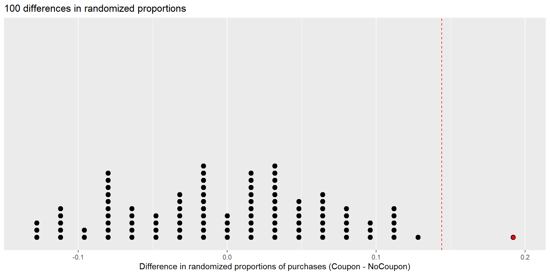
Dot plot of 100 differences in randomized proportions (null distribution), showing test statistic as dashed vertical line.
P-value
Dotplot with 1000 simulations has 16 dots is in the right tail, so the p-value is \(\frac{12}{1000}=0.012\)
Conclusion
In the consumer behavior example, the observed difference in proportions (\(\hat{p}_{Coupon}-\hat{p}_{NoCoupon} = 0.144\)) represents significant evidence against the null hypothesis (p-value = 0.012) at the \(\alpha = .05\) significance level.
So, our formal conclusion is that we reject the null hypothesis
The difference in the proportions is statistically significant
This means that there is strong evidence that offering the incentive of a 10% discount coupon significantly increased the probability of a purchase as compared with “no coupon” group.